Bundle
Excel Crash Course Exam (13 Sets) Questions with Verified Answers,100% CORRECT
13 Items

Excel Crash Course Exam 36 Questions with Verified Answers,100% CORRECT
Excel Crash Course Exam 36 Questions with Verified Answers
All of the following are keyboard shortcut that allow the user input to add more sheets to a ... [Show More] workbook EXCEPT:
Alt i w
Alt h i s
Shift F11
Alt Shift F1
Alt h i w
Incorrect - CORRECT ANSWER Alt i w, Alt h i s, Shift F11 and Alt Shift F1 are all keyboard shortcuts for adding more sheets to a workbook.
Alt h i w is not a valid shortcut.
What is a keyboard shortcut to open a file?
Ctrl o
Ctrl f
Alt o
Ctrl n - CORRECT ANSWER The correct answer is Ctrl o.
Ctrl f is the shortcut to find, or find and replace, text on the worksheet. Alt o is not a command. Ctrl n is the shortcut to open a new workbook.
What is the recommended workbook calculation setting for Excel?
Automatic
Manual
Automatic except for Data Tables
Iterate - CORRECT ANSWER The correct answer is "Automatic except for Data Tables".
Data tables can significantly slow down Excel and other programs. "Automatic", the default setting, will automatically calculate everything in the workbook, including data tables, which will make the program run more slowly. The Manual setting will require the user to frequently recalculate the workbook in order to display correctly. "Iterate" is not a setting for workbook calculation in Excel; iterative calculation is a toggle for users to set for workbooks that may have circular calculations.q
To add a cell reference from a different worksheet into an existing formula with your keyboard, you should follow the following steps:
1. Hit F2 to get into the existing formula; delete any incorrect formulas or operators 2. Hit F2 again to enable "Enter" mode on the bottom-left corner of the Excel sheet 3. Holding down Ctrl, use PageUp or PageDown to find the desired worksheet 4. Let go of the Ctrl and PageUp/Down keys 5. Use the arrow keys to locate the desired cell reference 6. Hit Enter
1. Hit F2 to get into the existing formula; delete any incorrect formulas or operators 2. Hit F2 again to enable "Enter" mode on the bottom-left corner of the Excel sheet 3. Holding down Alt, use PageUp or PageDown to find the desired worksheet 4. Let go of the Ctrl and PageUp/Down keys 5. Use the arrow keys to locate the desired cell reference 6. Hit Escape - CORRECT ANSWER The correct answer is:
Hit F2 to get into the existing formula; delete any incorrect formulas or operators
Hit F2 again to enable "Enter" mode on the bottom-left corner of the Excel sheet
Holding down Ctrl, use PageUp or PageDown to find the desired worksheet
Let go of the Ctrl and PageUp/Down keys
Use the arrow keys to locate the desired cell reference
Hit Enter
In the incorrect option, 3. Alt Page Up / Down will not allow the user to navigate to a different worksheet; 6. Hit Escape will not save any cell references, but will delete any new data or formula that has been entered into the cell.
What is the keyboard command to autofit the row height?
Alt o c a
Alt o c w
Alt h o h
Alt h o a - CORRECT ANSWER The correct answer is "Alt h o a"
Alt o c a is used to autofit column width. Alt o c w is used to assign the column width. Alt h o h is used to assign the row height.
What is the command to change the zoom size?
Alt v z
Alt t o v
Alt h o i
Alt h v t - CORRECT ANSWER The correct answer is "Alt v z".
Alt t o v is not a valid shortcut. Alt h o I is the shortcut to autofit the column width. Alt h v t is not a valid shortcut.
What is the keyboard shortcut to open the formatting cells dialog box?
Ctrl 1
Ctrl 2
Ctrl Shift 1
Ctrl Shift 2 - CORRECT ANSWER The correct answer is: Ctrl 1.
Ctrl 2 is not a valid shortcut. Ctrl Shift 1 is the shortcut to cycle through different number formats. Ctrl Shift 2 is the shortcut to cycle through different date formats.
What are the keyboard shortcuts for auto-fitting a range of columns?
1) Select the columns by hitting Ctrl Spacebar. 2) Hold down the shift key and use left and right arrow keys to highlight the range of columns. 3) Hit Alt H O I to auto fit the columns.
1) Hold down the shift key and use left and right arrow keys to select columns desired. 2) Hit Alt H O I to auto fit the columns
1) Select the columns by hitting Shift Spacebar. 2) Hold down the Ctrl key and use left and right arrow keys to highlight the range of columns. 3) Hit Alt H O W to auto fit the columns.
1) Select the columns by hitting Shift Spacebar. 2) Hold down the Shift key and use left and right arrow keys to highlight the range of columns. 3) Hit Alt H O W to auto fit the columns. - CORRECT ANSWER Select the columns by hitting Ctrl Spacebar.
Hold down the shift key and use left and right arrow keys to highlight the range of columns.
Hit Alt H O I to auto fit the columns.
Using the shift key and the right and left arrows will only autofit the column widths for the cells selected and will not apply autofit to all cells in the columns. Shift Spacebar will select a specific row rather than a specific column. Alt H O W will allow the user to select a specific column width but will not autofit the column width.
When you are in the Format Cells dialog (Ctrl 1):
What is the keyboard shortcut for moving across tabs (Number, Alignment, Font Border, Fill, Protection)?
How do you move counter clockwise across form elements?
How do you select a checkbox (put a checkbox next to it)
1) Tab 2) Ctrl Tab 3) Spacebar
1) Alt Tab 2) Ctrl Tab 3) Spacebar
1) Ctrl Tab 2) Shift Tab 3) Spacebar
1) Ctrl Tab 2) Shift Tab 3) Enter - CORRECT ANSWER The correct answer is: 1) Ctrl Tab 2) Shift Tab 3) Spacebar
Tab will navigate the user to different cells. Enter will keep the data the user has entered in the cell. Alt Tab is a shortcut to toggle among different Windows.
If I want to add the title "Company Financials" in cell A1 ensure that all columns are the same width across all the worksheets in my workbook, how would I do that?
1. Group the worksheets by hitting Ctrl Shift and use the left and/or right arrow keys to select the worksheets. 2. In the active sheet type in "Company Financials" in A1 and apply the desired width to all columns 3. Remember to hit Ctrl Pageup or Pagedown to make sure that future edits only apply to active sheet.
1. Group the worksheets by hitting Ctrl Shift and use the PageUp/Down keys to select the worksheets. 2. In the active sheet type in "Company Financials" in A1 and apply the desired width to all columns 3. Remember to hit Ctrl Pageup or Pagedown to make sure that future edits only apply to active sheet. - CORRECT ANSWER 1. Group the worksheets by hitting Ctrl Shift and use the PageUp/Down keys to select the worksheets. 2. In the active sheet type in "Company Financials" in A1 and apply the desired width to all columns 3. Remember to hit Ctrl Pageup or Pagedown to make sure that future edits only apply to active sheet.
What is the keyboard sequence to
1) Group highlighted columns (but not to hide group)
2) Hide the group (will show a + sign above the column)
3) Show the group (will show a + sign above the column)
1. Ctrl Alt Right Arrow 2. Alt a j 3. Alt a h
1. Ctrl Alt Right Arrow 2. Alt a h 3. Alt a s
1. Shift Alt Down Arrow 2. Alt a h 3. Alt a j - CORRECT ANSWER 1. Shift Alt Down Arrow 2. Alt a h 3. Alt a j
What is the keyboard shortcut to open the paste special dialog box?
Ctrl v
Ctrl e s
Alt e s or Alt h v s
Ctrl h v - CORRECT ANSWER The correct answer is: Alt e s or Alt h v s
Ctrl v is the shortcut for basic paste. Ctrl e s is not a valid shortcut sequence. Ctrl h v is not a valid shortcut sequence.
Which of the following keys IS NOT a way to trace precedent cells?
Ctrl [
Alt m p
Alt t u t
Ctrl Alt [ - CORRECT ANSWER The correct answer is: Ctrl [. Ctrl [ is not a valid shortcut. Alt m p, Alt t u t, and Ctrl Alt [ are all shortcuts that can be used to trace precedent cells.
What is the keyboard shortcut to freeze panes within a worksheet?
Alt F W V
Alt W S
Alt W F F
Alt A W T - CORRECT ANSWER The correct answer is: Alt w f f.
Alt f w v is the shortcut for Print Preview. Alt w s is the shortcut to split panes. Alt a w t is a shortcut to build data tables.
Please select the answer that best describes the shortcut to
Split (not freeze) an excel sheet into just two panes (top and bottom)
To navigate from pane to pane
1. Anywhere in the Excel worksheet hit Alt W S to split the panes to a top and bottom. 2. Hit F6 to jump from pane to pane (in some versions of Excel you will need to hit F6 several times to get from one pane to the other).
1. With the active cell on any row but in column A, hit Alt W S to split the panes to a top and bottom. 2. Hit F6 to jump from pane to pane (in some versions of Excel you will need to hit F6 several times to get from one pane to the other).
1. With the active cell on any column but in row 1, hit Alt W S to split the panes to a top and bottom. 2. Hit F6 to jump from pane to pane (in some versions of Excel you will need to hit F6 several times to get from one pane to the other). - CORRECT ANSWER The correct answer is:
With the active cell on any row but in column A, hit Alt w s to split the panes to a top and bottom.
Hit F6 to jump from pane to pane (in some versions of Excel you will need to hit F6 several times to get from one pane to the other).
If the active cell is not in Column A, the user will have more than 2 panes. If the active cell is in Row 1, the user will get two vertical panes.
You are in cell A1 and start a formula by typing = in a worksheet with split top and bottom panes. In order to jump to the bottom pane while working on the formula:
Hit Tab
Hit F6
Hit Alt F6
Hit Alt Tab - CORRECT ANSWER The correct answer is: Hit F6
Tab will navigate to the next cell. Alt F6 is not a valid shortcut. Alt Tab will navigate to a different window.
See lesson: Splitting & Freezing Panes
Identify the commands to insert a comment and delete a comment
1)Alt e m 2) Alt e m
1)Alt h e m 2) Alt I m
1)Shift F2 2) Alt h e m
1)Alt h e m 2) Alt I s - CORRECT ANSWER The correct answer is Shift F2, Alt h e m.
Alt e m is a shortcut to open the menu to move or copy a selected sheet. Alt I s is the shortcut to insert a symbol.
Identify the utility used to create a dropdown menu in Excel.
Alt d t
Alt d v l
Alt d l
Alt d d t - CORRECT ANSWER The correct answer is: alt d l.
Alt d t is the shortcut to build a data table. Alt d v l is not a valid shortcut. Alt d d t is not a valid shortcut.
Which of the following is NOT a shortcut for changing the format of a cell
Ctrl Tab
Ctrl Shift 1
Ctrl B
Alt h f c - CORRECT ANSWER The correct answer is Ctrl Tab.
Ctrl Tab will move the selected cell. It is not a shortcut used to format cells. Ctrl Shift 1 will change the cell to a Number format, Ctrl B makes the cell text bold, Alt h f c will allow to change the text color.
Identify the shortcut to remove arrows from Trace Precedents or Trace Dependents.
Alt d t
Alt m p
Alt m d
Alt m a - CORRECT ANSWER The correct answer is Alt m a.
Alt d t inserts a data table. Alt m p is the shortcut to trace precedents. Alt m d is the shortcut to trace dependents.
Identify a function in cell D6 that will return the fraction of the year elapsed assuming a 360 day count basis.
=STUB(D4,D5)
=YEARFRAC(D4,D5,2)
=DAYS360(D4,D5)
=YEARFRAC(D4,D5) - CORRECT ANSWER The correct answer is: =YEARFRAC(D4,D5,2). STUB is not an Excel formula. DAYS360 will return the number of days in a 360 day year. YEARFRAC(D4,D5) will calculate the fraction using a 365-day year.
Identify the formula that will always output a date that is the end-of-month date 3 months after the date inputted in D5.
=DATE(YEAR(D5),MONTH(D5)+3,DAY(D5))
=EOMONTH(3,D5)
=EOMONTH(D5,3) - CORRECT ANSWER The correct answer is: =EOMONTH(D5,3)
=DATE(YEAR(D5),MONTH(D5)+3,DAY(D5)) will add 3 months to the data inputted in D5. EOMONTH(3,D5) reverses the arguments required for this function.
Identify the formula that, based in user inputs in cells B1 and B2, outputs the text "animal lover" for users who have at least 1 dog and at least one cat, and outputs "lonely person" when those conditions are not met.
=IF(OR(B1>0,B2>0),"animal lover","lonely person")
=IF(AND(B1>1,B2>1),"animal lover","lonely person")
=IF(AND(B1>0,B2>0),"animal lover","lonely person")
=AND(IF(B1>0,"animal lover","lonely person"),IF(B2>0,"animal lover","lonely person")) - CORRECT ANSWER The correct answer is: =IF(AND(B1>0,B2>0),"animal lover","lonely person")
=IF(OR(B1>0,B2>0),"animal lover","lonely person") will output "animal lover" if the user owns a dog OR a cat.
=IF(OR(B1,B2>0),"animal lover","lonely person") is not valid formula syntax.
=AND(IF(B1>0,"animal lover","lonely person"),IF(B2>0,"animal lover","lonely person")) is not valid formula syntax.
What IF function will output revenue growth based on the Scenario selected in cell F10?
=IF(F10=C14,F14,IF(F10=C15,F15,F16))
=IF(F10=C15,F15,IF(F10=C14,F14,F16))
=IF(F10=C16,F16,IF(F10=C14,F14,F15))
All of the above - CORRECT ANSWER The correct answer is: All of the above.
This question uses a nested IF statement. Any of the cases (Best case, Base case, Weak case) can be used as the logical test, which is the first argument in the IF statement. Two IF statements are required because there are thee possible scenarios. The last argument in the function will have the case that was not used in the two logical tests. These logical tests can be in any order.
Identify the best formula that will output 2016 expenses. Hint: Only select the 'range lookup' argument if it is necessary.
=HLOOKUP(2016,B2:D4,2,0)
=HLOOKUP(2016,A1:D4,3)
=HLOOKUP("Expenses",A1:D4,2)
=HLOOKUP(2016,B2:D4,2) - CORRECT ANSWER The correct answer is: =HLOOKUP(2016,A1:D4,3)
=HLOOKUP(2016,B2:D4,2,0) will not result in a valid output because 2016 is not selected in the table array argument.
=HLOOKUP("Expenses",A1:D4,2) will result in a #NAME error because "Expenses" is not a horizontal lookup reference.
=HLOOKUP(2016,B2:D4,2) will reference the Revenue line rather than the expenses line because the third argument references the row 2 in the table array.
Identify the formula that will output 2016 expenses (55).
=OFFSET(B1,3,2)
=OFFSET(B1,2,3)
=OFFSET(A1,2,2)
=OFFSET(A1,3,3) - CORRECT ANSWER The correct answer is: =OFFSET(A1,2,2)
=OFFSET(B1,3,2) will return 65.
=OFFSET(B1,2,3) will return (75).
=OFFSET(A1,3,3) will return 55.
Identify the formula that will output 2016 expenses:
=CHOOSE(2,B3:D3)
=CHOOSE(2,B3,C3,D3)
=CHOOSE(2,A3,B3,C3,D3) - CORRECT ANSWER The correct answer is: =CHOOSE(2,B3,C3,D3)
=CHOOSE(2,B3:D3) is not valid syntax for this formula; cells must be individually selected.
=CHOOSE(2,A3,B3,C3,D3) will output 2015 expenses.
Identify the formula that outputs 2016 expenses.
=VLOOKUP("Expenses",A1:D4,3,1)
=VLOOKUP("Expenses",A1:D4,3)
=VLOOKUP(2016,A1:D4,3)
=VLOOKUP("Expenses",A1:D4,3,0) - CORRECT ANSWER The correct answer is: =VLOOKUP("Expenses",A1:D4,3,0)
=VLOOKUP("Expenses",A1:D4,3,1) looks for an approximate match and requires that the reference range be in ascending order.
=VLOOKUP("Expenses",A1:D4,3) also looks for an approximate match as specified by match type 1, and requires that the reference range be in ascending order.
Identify the formula that outputs data from the table based on the user inputs in cells C6 and C7.
=OFFSET(A1,MATCH(C6,A2:A4),MATCH(C7,B1:D1))
=OFFSET(B1,MATCH(C6,A2:A4,0),MATCH(C7,B1:D1))
=OFFSET(A1,MATCH(C6,A2:A4,0),MATCH(C7,B1:D1))
=OFFSET(A1,MATCH(C7,B1:D1),MATCH(C7,A2:A4,0)) - CORRECT ANSWER The correct answer is: =OFFSET(A1, MATCH(C6,A2:A4,0),MATCH(C7,B1:D1)).
=OFFSET(A1,MATCH(C6,A2:A4),MATCH(C7,B1:D1)) does not return the correct value because an exact match is not specified for the MATCH function used for the 'row' argument of the OFFSET function.
=OFFSET(B1,MATCH(C6,A2:A4,0),MATCH(C7,B1:D1)) uses an incorrect cell reference for the reference argument of the OFFSET function, which must be in the upper left corner of the table.
=OFFSET(A1,MATCH(C7,B1:D1),MATCH(C7,A2:A4,0)) reverses the MATCH functions used for the row and column references in the OFFSET function, returning #N/A.
What INDEX & MATCH combo will create a dynamic reference based on whatever metric and date you input in cells F10 and F11, respectively?
=INDEX(D6:H8,MATCH(F10,C6:C8,0),MATCH(F11,D5:H5,0))
=INDEX(D6:H8,MATCH(F10,C6:C8,1),MATCH(F11,D5:H5,0))
=INDEX(D6:H8,MATCH(F10,C6:C8,1),MATCH(F11,D5:H5,1))
=INDEX(D6:H8,MATCH(F10,C6:C8,0),4) - CORRECT ANSWER The correct answer is: =INDEX(D6:H8,MATCH(F10,C6:C8,0),MATCH(F11,D5:H5,0)).
=INDEX(D6:H8,MATCH(F10,C6:C8,1),MATCH(F11,D5:H5,0)) uses match type 1 for the first argument, which requires values to be in ascending order, and is not valid for this reference.
=INDEX(D6:H8,MATCH(F10,C6:C8,1),MATCH(F11,D5:H5,1)) uses match type 1 for both MATCH function, which requires values to be in ascending order, and is not valid for this reference.
=INDEX(D6:H8,MATCH(F10,C6:C8,0),4) selects the fourth column instead of the fifth, and is static; it will not change if a different date is entered.
Below is a Data Table designed to display the effect on 2015 Net Profit based of changes in 2015 Revenue Growth and 2015 COGS %. Please provide:
The cell reference required in D22.
The row input cell required by the Data Table.
The column input cell required by the Data Table.
Provide all three cell references, in order above, separated by commas with no space (i.e. A1,A2,A3) Note: Do not include spaces within answer - CORRECT ANSWER The correct answer is: E8,E10,E11
E8 is the cell reference for 2018 Net Income, the output variable, which must be in the top left corner of the table. E10, the 2015 revenue growth rate, is the row input cell, the variable that is being sensitized in the top row of the table. E11, the COGS %, is the column input variable that is being sensitized.
Identify the formula that sums the property values of properties in Boston.
=SUMIF(B2:B5,"Boston",C2:C5)
=SUMIF(C2:C5,"Boston",B2:B5)
=SUMIF(C2:C5,Boston,B2:B5) - CORRECT ANSWER The correct answer is: =SUMIF(C2:C5,"Boston",B2:B5)
=SUMIF(B2:B5,"Boston",C2:C5) does not use the correct range for matching with the sum criteria
=SUMIF(C2:C5,Boston,B2:B5) does not use quotes for "Boston", which will return an error
Identify the formula that outputs the sum of property values for properties in Boston that were built after 1950.
=SUMIFS(B2:B5,C2:C5,"Boston",D2:D5,">1950")
=SUMIFS(C2:C5,"Boston",D2:D5,">1950",B2:B5)
=SUMIF(B2:B5,and(D2:D5,">1950",C2:C5,"Boston") - CORRECT ANSWER The correct answer is: =SUMIFS(B2:B5,C2:C5,"Boston",D2:D5,">1950")
=SUMIFS(C2:C5,"Boston",D2:D5,">1950",B2:B5) selects column C instead of Column B as the sum range
=SUMIF(B2:B5,and(D2:D5,">1950",C2:C5,"Boston") incorrectly selects column D instead of column B as the sum range
What formula using a "sum" function returns the correct value for the proceeds for options "in the money" as seen in cell C11 (i.e., maximum proceeds for options with a strike price less than the share price)? - CORRECT ANSWER The correct answer is: =SUMPRODUCT(B5:B9,C5:C9*(C5:C9
- Exam
- $10.45
- 0
- 46

Excel Crash Course Exam 128 Questions with Verified Answers,100% CORRECT
Excel Crash Course Exam 128 Questions with Verified Answers move back and forth between the worksheets in a workbook - CORRECT ANSWER *Ctrl PageUp* or *... [Show More] Ctrl PageDown* open a file - CORRECT ANSWER *alt f o* *ctrl o* save a file - CORRECT ANSWER *alt f s* *ctrl s* print a file - CORRECT ANSWER *alt f p* *ctrl p* navigating to the toolbars without the mouse - CORRECT ANSWER hit *Alt and the appropriate letter* (or use the right/left arrow keys) to get to the desired tab once there, use the Tab and Shift Tab keys to navigate around accessing settings - CORRECT ANSWER File > Options (*Alt f t*) *Alt t o* Disabling the Start Screen and adding more worksheets on startup - CORRECT ANSWER click on 'Blank worksheet' Hit *Alt f t* go go to Excel options (you can also get there by clicking the file tab) Under 'General' unselect "Show the Start screen when this application starts" password protecting files - CORRECT ANSWER File Info password protect files: "Encrypt with Password" password protect individual worksheet (so that people can't see or edit formulas): "Protect Current Sheet" highlighting columns and rows - CORRECT ANSWER columns: *Ctrl Spacebar* rows: *Shift Spacebar* widening columns and rows - CORRECT ANSWER highlight column by pressing *Ctrl Spacebar* *Alt h o i* to auto-fit the column width -if you want a column to have a certain width, press *Alt h o w* and enter the desired width highlight row by pressing Shift Spacebar *Alt h o a* to auto-fit the row height -if you want a row to have a certain height, press *Alt h o h* and enter the desired height format cells - CORRECT ANSWER *Ctrl 1* pulls up the 'Format Cells' menu navigating the 'Format Cells' menu - CORRECT ANSWER after hitting Ctrl 1 to pull up the 'Format Cells' menu, you can navigate around tabs by hitting *Ctrl tab* each category within a tab can be accessed by pressing *Alt* and the appropriate underlined letter, or by hitting *tab* to move clockwise and *shift tab* to move counter clockwise when on the desired tab, horizontal alignment can be accessed through *Alt h* and vertical alignment through *Alt v* paste special - CORRECT ANSWER *Alt v s t* or *Alt e s t* changing zoom size - CORRECT ANSWER *Alt w q* or *Alt v z* Move/copy a tab - CORRECT ANSWER *Alt h o m* freezing panes - CORRECT ANSWER click the cell BELOW the desired row and to the RIGHT of the desired column where you want to freeze panes and hit *Alt w f f* to unfreeze panes: press *Alt w f f* again splitting panes - CORRECT ANSWER splitting panes allows users to scroll in both areas of the worksheet, while rows and columns in the non-scrolled area remain visible to split panes: -click the cell BELOW the desired row and to the RIGHT of the desired column where you want to split panes and hit *Alt w s* -to unspilt panes, click *Alt w s* again -press *F6* to move from pane to pane in a clockwise direction; press *Shift F6* to move from pane to pane in a counter-clockwise direction manipulating data inside a cell - CORRECT ANSWER *F2* is the command that puts you inside a cell: -pressing the F2 key once shows you the components of the formula you created earlier, puts you inside a cell and enables you to navigate through it to edit the existing cell data -pressing the F2 key twice activates the cursor and enables you to move to different cells, worksheets, and even other open Excel files *Shift arrow key* will highlight characters one at a time *Shift Ctrl arrow key* will highlight contiguous ranges of characters deleting and clearing cell data - CORRECT ANSWER hitting *Delete* does NOT delete the formatting in the cell to truly delete a cell: -*Alt h e* (Home tab > Clear) -from the drop-down, chose the appropriate actions *(Alt h e) a*: clears ALL contents of the cell *(Alt h e) f*: clears only the cell FORMAT *(Alt h e) c*: clears only the cell CONTENT -this is the same as hitting Delete *(Alt h e) m*: clears only the cell COMMENTS right and down fills - CORRECT ANSWER highlight the range *Ctrl R* tells Excel to look at the LEFTMOST column of a range of highlighted cells and copy and paste the inputs and formulas in that column to all the columns to the right *Ctrl D* does the same thing for rows that Ctrl R does for columns, telling Excel to look at the topmost row of a range of highlighted cells and to copy and paste the inputs and formulas in that row down to all the rows below it inserting comments - CORRECT ANSWER enter the cell and type *Shift F2* hit *Esc* twice to exit the comment area to edit an existing comment: go to the cell and press *Shift F2* to delete a comment: press *Alt h e am* inserting rows - CORRECT ANSWER highlight the row BELOW the row where you want to add a row press *Shift spacebar* to highlight the entire row press *Ctrl Shift +* to insert the row note: Excel will insert the row ABOVE the row that is highlighted inserting columns - CORRECT ANSWER *Ctrl Spacebar* to highlight the entire column *Ctrl Shift +* to insert the column note: Excel will insert the row to the LEFT of the column that is highlighted deleting rows and columns - CORRECT ANSWER row: *Alt h d r* column: *Alt h d c* OR highlight row/column and press *Ctrl -* Paste special - transpose - CORRECT ANSWER this feature allows users to convert a vertical list of data into a horizontal list of data, and vice versa highlight the vertical list of data in an open cell, press *Alt e s e* -your vertical list of data should now be listed horizontally *Ctrl Shift !* - CORRECT ANSWER number format: 2 decimals, 000 separator *Ctrl Shift $* - CORRECT ANSWER currency format: 2 decimal places *Ctrl Shift %* - CORRECT ANSWER percentage format with no decimal places *Ctrl Shift #* - CORRECT ANSWER date format with the day, month, and year *Ctrl Shift _* - CORRECT ANSWER remove all borders anchoring cells - CORRECT ANSWER when you copy and paste a cell containing a formula from one cell to another, Excel automatically shifts the cells being referenced in the formula sometimes this is not desirable, which is why Excel allows you to anchor cells Anchoring (or "Fixing") cells that are being referenced in a formula tells Excel that even if you copy the formula to another cell, the cells in the formula that are anchored should not change fix column: $ before letter fix row: $ before number fix entire cell: $ before letter and before number renaming a worksheet you are working in - CORRECT ANSWER *Alt h o r* inserting and deleting worksheets - CORRECT ANSWER add a new worksheet: *Alt h i s* or *Alt i w* delete a worksheet: *Alt e l* new tab - CORRECT ANSWER *Shift F11* Grouping columns and rows - CORRECT ANSWER to group columns: -hit *Ctrl Spacebar* to select the desired column(s) -hit *Shift Alt right arrow key* to create the group -hitting *Alt a h* will hide the columns -hitting *Alt a j* will unhide the columns -hitting *Shift Alt left arrow key* will remove the group to group rows: -hit *Shift Spacebar* to select the desired rows -follow the other steps above grouping vs hiding - CORRECT ANSWER another way to hide data is by hitting *Alt h o u r* for rows and *Alt h o u c* for columns, but don't ever use this method because under this method, columns and rows are hidden, but there are no indications (no minus or plus signs as in the first method) as to their location so it's easy to forget which columns and rows you've hidden grouping worksheets - CORRECT ANSWER if you want to format data in the same manner or enter the same data across multiple sheets, Excel allows you to do this by grouping multiple worksheets, any data and formatting that you would perform in one of the grouped worksheets would automatically be reflected in all of them to group worksheets: -holding down *Ctrl Shift*, press *PageUp* or *PageDown* to reach the worksheets you would like to group -all of the grouped worksheets are highlighted and the file name on top of the Excel screen should show [Group] after it to ungroup worksheets - CORRECT ANSWER press *Ctrl PageUp* or *Ctrl PageDown* until you reach one of the ungrouped worksheets; this automatically groups all of the previously grouped sheets auditing cells - CORRECT ANSWER go to the cel and hit F2 OR hitting *Ctrl [* on a cell will highlight the precedent cells -keep hitting *Ctrl [* and it will take you to the next precedent, and on and on hitting *Ctrl ]* on a cell will do the same thing but for dependent cells Excel's formula auditor - CORRECT ANSWER trace precedents: *Alt m p* -to trace cells that provide data to a formula -a worksheet icon indicates that the precedent cells are in another worksheet -double clicking anywhere with a mouse on the black arrow brings up the 'Go To' screen; selecting either of the precedent cell locations and hitting 'Ok' will take you there trace dependents: *Alt m d* -to trace formulas that reference a particular cell (the cell highlighted) remove trace arrows: *Alt m a a* evaluate formula - CORRECT ANSWER *Alt m v* track changes - CORRECT ANSWER *Alt r g* zoom to selection - CORRECT ANSWER *Alt w g* "go to" - CORRECT ANSWER *F5* Error: formula treated as text - CORRECT ANSWER forgetting the equal sign (=) at the start or inserting a space before the equal sign of the formula is created by Excel as text Error: #Div/0! - CORRECT ANSWER dividing a number by 0 Error: #REF! - CORRECT ANSWER an invalid cell reference Error: #NUM! - CORRECT ANSWER inserting invalid numerical values in a formula or function Error: #NAME? - CORRECT ANSWER unrecognizable text in a formula Error: #VALUE! - CORRECT ANSWER inserting incorrect arguments in a function Error: ##### - CORRECT ANSWER when the column is not wide enough to fit the data in a cell you must widen the cell to fix the error (*Alt h o i*) logical functions: IF - CORRECT ANSWER the IF function returns one value if a condition you specify evaluates to TRUE, and another value if it evaluates to FALSE IF statements follow the same structure = IF(x,y,z) where: x: criteria y: output if criteria evaluates to true z: output if criteria evaluates to false text output is designated by quotation marks around the outputs error-trapping function IFERROR - CORRECT ANSWER =IFERROR(value, value_if_error) returns a value you specify if a formula evaluates to an error. If the formula does not result in an error, IFERROR returns the result of the formula creating dynamic headers by combining cell references with text ("&") - CORRECT ANSWER Excel allow users to combine (or "concatenate") cells with a text string in them with other text strings, creating one text string by using the "&" function EOMONTH - CORRECT ANSWER =EOMONTH(start_date, months) allows you to create monthly date headers, by outputting the last day of a specified month start_date: represents a starting date reference months: represents x number of months before or after the start_date to output a date x months before a start_date, x should be negative EDATE - CORRECT ANSWER =EDATE(start_date, months) similar to EOMONTH, but the difference is that EDATE returns the exact date, x months from the start date YEARFRAC - CORRECT ANSWER =YEARFRAC(start_date, end_date, basis) returns the proportion of the year between two given dates (the start_date and the end_date) basis is an optional parameter that represents the number of days per month/year used to calculate the proportion of the year: 0 or omitted: US 30/360 1: actual/actual 2: actual/360 3: actual/365 4: European 30/360 DATE - CORRECT ANSWER =DATE(year, month, date) is a function that combines distinct year, month, and day elements into a valid date function in Excel combining this function with DAY(serial number), MONTH(serial number), and YEAR(serial number) is sometimes helpful for creating date functions out of disparate data cell contents as criteria in IF statements - CORRECT ANSWER a surprisingly useful criteria used in IF statements is a test of whether a cell has anything in it ex: the IF statement =IF(C1, C2, C3) would see if there is anything in cell c1, and if there was, it would output C2, otherwise C3 ISNUMBER and ISTEXT - CORRECT ANSWER both typically embedded within an IF statement, they test whether there is number or text inside a cell, respectively AND - CORRECT ANSWER =AND(logical1, logical2,...) evaluates to true if all of its arguments are true; false if one or more arguments is false OR - CORRECT ANSWER =OR(logical1, logical2,...) evaluates to true if at least one argument is true HLOOKUP - CORRECT ANSWER =HLOOKUP(lookup_value, table_array, row_index_number, [range_lookup]) searches for a value in the top row of a table or an array of values, and then returns a value in the same column from a row you specify in the table/array use HLOOKUP when your comparison values are located in a row across the top of a table of data, and you want to look down a specified number of rows VLOOKUP - CORRECT ANSWER =VLOOKUP(lookup_value, table_array, col_index_num, range_lookup) searches for a value in the LEFTMOST column of a table and then returns a blue in the same row from a column you specify the table/array use VLOOKUP when your comparison values are located in a column to the left of a table of data, and you want to look across (and to the right) a specified number of columns range_lookup - CORRECT ANSWER TRUE: an approximate match to the lookup value is returned FLASE: an exact match is returned when lookup value is text or numbers is non-ascending order, the FALSE range is often preferred OFFSET - CORRECT ANSWER =OFFSET(reference, rows,cols,height,width) returns a cell value or range of cell values that is a specified number of rows and columns from a cell or range of cells INDEX - CORRECT ANSWER =INDEX(array, row_num, column_num) returns a value from a specified row and column from within a table or range CHOOSE - CORRECT ANSWER =CHOOSE(index_num, value1, value2, value3,...) returns a number from a specified list of up to 254 values MATCH - CORRECT ANSWER =MATCH(lookup_value,lookup_array,match_type) returns the relative position (number) of an item in an array that matches the specified lookup value it does NOT return the value within the cell itself (as opposed to the HLOOKUP and VLOOKUP functions) data validation - CORRECT ANSWER data validation is a utility in Excel, whose most frequently used feature is its ability to create simple and quick drop-down menus to create a drop down menu: -with the cell where you want your drop down menu active, open the data validation form (*Alt d l* -within the Settings tab, select list from the dropdown menu -within the 'Source' field, identify a contiguous cell range containing the data you want to include in your dropdown, and hit OK and you should your dropdown menu appear note: it only appears when you are on the active cell building a vertical data table - CORRECT ANSWER 1. identify the output variable -the variable you are trying to sensitize is the output variable -must be referenced from your analysis into the TOP RIGHT CORNER of the data table 2. hard-code the input variable sensitivities -the variables whose impact on the output variables you want to analyze are the input variables -input variable assumptions should not be referenced from the analysis, but rather be hard-coded and arranged in the column to the right of the output variable 3. run the data table -hit *Alt d t*: the Data Table dialog will appear row input cell: not needed for vertical data tables column input cell: reference the input variable from the model -highlight the entire range (including the output variable) and hit OK when done - the data table should populate -you. may need to hit *F9* if Excel is set to "manual" or "automatic calculations except for data tables" NOTE: data tables must always be in the same worksheet as the input variables building a horizontal data table - CORRECT ANSWER 1. referenced output variable from your analysis into the BOTTOM LEFT CORNER of your data table 2. input the input assumptions in the row above and one cell to the right of the output reference 3. highlight the entire range (including the output variable) and hit *Alt d t*: the Data Table dialog will appear row input cell: reference the input variable from the model column input cell: not needed 4. hit OK when done - the data table should populate building a 2-sided data table - CORRECT ANSWER same as vertical data table, but allows for 2 inputs instead of one output variable must be referenced from the model into the TOP LEFT CORNER of the data table now both row input cell and column input cell are needed SUMPRODUCT - CORRECT ANSWER =SUMPRODUCT(array1,array2,array3,...) multiplies corresponding components in two or more arrays, and returns the sum of those products Booleans in Excel - CORRECT ANSWER when Excel spits out a TRUE or FALSE, you can convert them respectively into 1 or 0 by applying any operator on them multiply the TRUE/FALSE cell by 1: will convert a TRUE to 1 and FALSE to 0 multiply the TRUE/FALSE cell by TRUE: will convert a TRUE to 1 and FALSE to 0 SUMIF - CORRECT ANSWER =SUMIF(range, criteria, sum range) adds the cells specified by a given criteria criteria can either be hardcoded (which requires quotation marks) or a direct cell reference (which does not need quotation marks) SUMIFs - CORRECT ANSWER =SUMIF(range1, criteria1, sum range1, range2, criteria2, sum range2, etc.) same as SUMIF but can handle multiple criteria and sum ranges AVERAGEIF and AVERAGEIFs - CORRECT ANSWER identical to SUMIF and SUMIFS but instead of summing, this function averages the data in the range ABS, CEILING, FLOOR - CORRECT ANSWER ABS(cell) returns the absolute value of that cell CEILING(cell, x) rounds input cell up to nearest x FLOOR (cell, x) rounds input down to nearest x COMBIN - CORRECT ANSWER Returns the number of combinations for a given number of objects useful accounting application: sum of years' digits n(n+1)/2 =COMBIN(cell+1,2) ROUND, ROUNDUP, ROUNDDOWN - CORRECT ANSWER ROUND: rounds most accruately ROUNDUP: rounds up ROUNDDOWN: rounds down MIN and MAX - CORRECT ANSWER =MIN(number1,number2,...) returns the smallest number in a specified set of values) =MAX(number1,number2,...) returns the largest number in a specified set of values COUNT - CORRECT ANSWER =COUNT(value1, value2,...) counts the number of cells that contain numbers within the list of arguments -cells with text are disregarded COUNTA - CORRECT ANSWER same as COUNT except cells with numbers and text are counted COUNTIF - CORRECT ANSWER =COUNTIF(range, criteria) counts the number of items in the range that satisfy a specific criteria -similar to the SUMIF function COUNTIFS - CORRECT ANSWER allows for multiple criteria -similar to the SUMIFS function PV function - CORRECT ANSWER returns the present value of a series of future payments =PV(rate, nper, pmt, fv, type) rate: interest rate per period nper: total number of payment periods pmt: payment made during each period (it cannot change) fv: future value type: indicates when payments are due (0 or omitted = end of period, 1 = beginning of period) FV function - CORRECT ANSWER returns the future value of an investment based on constant payment and interest rate =FV(rate, nper, pmt, pv, type) rate: interest rate per period nper: total number of payment periods pmt: payment made during each period (it cannot change) pv: present value type: indicates when payments are due (0 or omitted = end of period, 1 = beginning of period) NPV function - CORRECT ANSWER =NPV(rate, value1, value 2, ...) returns the net present value of an investment based on a discount rate and a series of future payments (negative values) and income (positive values) values are assumed to occur at the end of each time period and must be referenced in the order in which they occur NPV vs. PV functions - CORRECT ANSWER PV assumes constant payments, while NPV cash flows can vary from period to period NPV does not require the user to explicitly identify number of periods and simply assumes equal periods based on the number of values NPV assumes payments occur at the end of the period (but formula can be adjusted to simulate payments accusing at beginning of period) XNPV function - CORRECT ANSWER NPV performs equal discounting on each cash flow =XNPV(rates, values, dates) returns the net present value for a set of cash flows that don't necessarily occur t equal time intervals unlike NPV, the first cash flow is not discounted, while dates of subsequent cash flows can be included in the formula in any order IRR - CORRECT ANSWER =IRR (values, guess) returns the IRR for a series of values IRR is the rate corresponding to an NPV of 0 while values don't have to be identical each period, the periods are assumed to be equally far apart 'Guess' is an optional argument: Excel needs a starting point to iterate to the right IRR; if you don't input a guess, Excel will automatically use 10% as the guess note: there must be both positive and negative values XIRR - CORRECT ANSWER =XIRR(values, dates, guess) returns the IRR for a series of values which may not be periodic the date of each cash flow must be referenced in the formula (the "dates") note: there must be both positive and negative values Flash Fill - CORRECT ANSWER *Ctrl e* sorting data - CORRECT ANSWER *Alt d s* (Data tab > Sort) combining Sort & Subtotal - CORRECT ANSWER Subtotal: *Alt a b* autofiltering - CORRECT ANSWER *Alt a t* the filtered rows get hidden but not deleted if you copy and paste the filtered range to another area of the worksheet or a different worksheet, id doesn't copy over the hidden rows once a filter is applied, you can tell which column was filtered via the funnel icon to remove individual filters, click on the filter icon and "Clear filter" to remove all filters, hit *Alt a t* again pivot tables - CORRECT ANSWER select any cell inside the table of data and hit *Alt n v* -Excel will automatically highlight the entire table of data -select to open the Pivot Table in a new worksheet a new worksheet will open showing the Pivot Table Field List -this shows a list of the data's categories and the 4 areas of the Pivot Table (filters, columns, rows, values) using your mouse, you can drag any of the data categories into any of the 4 areas of the Pivot Table -as you drag a category into one of the 4 areas of the table, the Pivot Table itself will automatically reorganize to accommodate the newly added category value field settings (pivot tables) - CORRECT ANSWER VALUES > Field Settings the Field Settings enables you to show outputs in a variety of different ways (ex: to see counts instead of sums) the Value Field Settings also has a "Show Values As" tab, which enables you to present the VALUES in a variety of useful ways recording macros - CORRECT ANSWER rather than repeatedly going through the same series of steps, Excel allows you to record a sequence of instructions, and assign a keyboard shortcut to invoke them as desired -these instructions are called macros 1. select 'Use Relative References' 2. place the cursor in any cell 3. *Alt l r* brings up "Record Macro" menu 4. input a name and shortcut key (ex: ctrl shift z) -as soon as you hit "OK" you are starting to record this macro 5. format the cell 6. when finished, hit *Alt l r* to stop recording now if you go to any other cell and enter the shortcut you inputted (in this case ctrl shift z), those cells' contents should be formatted per your preferences repeat - CORRECT ANSWER *Ctrl Y* Outline border - CORRECT ANSWER *Shift Ctrl &* toggle Excel workbooks - CORRECT ANSWER *Ctrl tab* Min/restore ribbon - CORRECT ANSWER *Ctrl F1* print preview - CORRECT ANSWER *Ctrl F2* close window - CORRECT ANSWER *Ctrl F4* move to cell "A1" - CORRECT ANSWER *Ctrl Home* move to cell above - CORRECT ANSWER *Shift Enter* move to cell to the right - CORRECT ANSWER *tab* move to cell to the left - CORRECT ANSWER *Shift Tab* show formulas/values - CORRECT ANSWER *Ctrl ~* fill selection with entry - CORRECT ANSWER *Ctrl enter* recalculate all workbooks - CORRECT ANSWER *F9* get inside a drop-down list - CORRECT ANSWER *Alt + up/down arrow key* display "Insert Function" box - CORRECT ANSWER *Alt I F (Shift F3)* display "Name" box - CORRECT ANSWER *Ctrl F3* Enter array formula - CORRECT ANSWER *Shift Ctrl Enter* replace - CORRECT ANSWER *Ctrl H* insert AutoSum formula - CORRECT ANSWER *Alt +" (hold down Alt) start a new line in same cell - CORRECT ANSWER *Alt Enter* Welcome to Excel: -Shortcuts (New Sheet) - CORRECT ANSWER SHIFT + FN11 Welcome to Excel: -Shortcuts (Auto Column Width) - CORRECT ANSWER ALT HOI Welcome to Excel: -Shortcuts (Customize Column Width) - CORRECT ANSWER ALT HOW *think W for Width Welcome to Excel: -Shortcuts (Customize Row Height) - CORRECT ANSWER ALT HOH *think H for Height Welcome to Excel: -Shortcuts (Highlight column) - CORRECT ANSWER CTRL + SPACE Welcome to Excel: -Shortcuts (Highlight row) - CORRECT ANSWER SHIFT S+ SPACE Welcome to Excel: -Shortcuts (Formatting cells) - CORRECT ANSWER CTRL + 1 Welcome to Excel: -Shortcuts (Highlighting cells that are hardcoded) - CORRECT ANSWER FN5 ALT + S Constants --> unclick "Text" [Show Less]
- Exam
- $11.45
- 0
- 46

Excel Exam 62 Questions with Verified Answers,100% CORRECT
Excel Exam 62 Questions with Verified Answers spreadsheet - CORRECT ANSWER an electronic file that contains a grid of columns and rows containing relate... [Show More] d data worksheet - CORRECT ANSWER s spreadsheet that contains formulas, functions, values, texts, and visual aids workbook - CORRECT ANSWER a file containing related worksheets input area - CORRECT ANSWER a range of cells containing values for vairables used in formulas output - CORRECT ANSWER a range of cells containing results based on manipulating the variables name box - CORRECT ANSWER identifies the address of the current cell formula bar - CORRECT ANSWER displays the content (text, value, date, or formula) in the active cell sheet tab - CORRECT ANSWER diplays the name of a worksheet within a work-book cell - CORRECT ANSWER the interesection of a column letter and a row number cell address - CORRECT ANSWER identifies a cell by a letter and a ro number active cell - CORRECT ANSWER the current cell, indicated by a dark border text - CORRECT ANSWER includes letters, numbers, symbols, and spaces value - CORRECT ANSWER a number that represents a quantity or an account formula - CORRECT ANSWER a combination of cell refrences, operators, values, and or functions used to perfom a calculation range - CORRECT ANSWER a rectangular group of cells nonadjacent range - CORRECT ANSWER contains multiple ranges of cells semi-selection - CORRECT ANSWER the process of using the mouse pointer to select cells while building a formula relative cell reference - CORRECT ANSWER indicates a cell's relative location from the cell containing the formula, the cell reference changes when the formula is copied absolute cell reference - CORRECT ANSWER indicates a cell's specific location; the cell reference does not change when you copy the formula mixed cell reference - CORRECT ANSWER contains both an absolute and a relative cell reference in a formula; the absolute part does not change but the relative part does when you copy the formula circular reference - CORRECT ANSWER occurs when a formula directly or indirectly refers to itself syntax - CORRECT ANSWER a set of rules that govern the structure and components for properly entering a function arguement - CORRECT ANSWER an input, such as a cell reference or value, needed to complete a function function screentip - CORRECT ANSWER a small pop-up description that displays the arguements for a function as you enter it counta function - CORRECT ANSWER tallies the number of cells in a range that are not empty now function - CORRECT ANSWER displays current date and time if function - CORRECT ANSWER evaluates a condition and returns one value if the condition is true and a different value if the conditon is false logical test - CORRECT ANSWER an expression that evaluates to true or false nested function - CORRECT ANSWER a function that contains another function embedded inside one or more of its arguements vlookup function - CORRECT ANSWER looks up a value in a vertical lookup table and returns a related result from the lookup table table array - CORRECT ANSWER a range containing a lookup value pmt function - CORRECT ANSWER calculates the periodic payment for a loan with a fixed interest rate and fixed term rate - CORRECT ANSWER the periodic interest rate, such as a monthly interest rate nper - CORRECT ANSWER the number of total payment periods pv - CORRECT ANSWER the present value of the loan range name - CORRECT ANSWER a word or string of characters that represents one or more cells column chart - CORRECT ANSWER displays data comparisons vertically in columns chart area - CORRECT ANSWER contains the entire chart and all of its elements plot area - CORRECT ANSWER contains a graphical representation of values in a data series value axis - CORRECT ANSWER displays incremental values to identify the values of the data series legend - CORRECT ANSWER a key that identifies the color, gradient, picture, texture, or pattern fill assigned to each data series in a chart stacked column chart - CORRECT ANSWER places stacks of data in segments on top of each other in on column, with each category in the data series represented by a different color bar chart - CORRECT ANSWER compares values across categories using horizontal bars line chart - CORRECT ANSWER uses a line to connect data points in order to show trends over a period of time sparkline - CORRECT ANSWER a miniature chart contained in a single cell chart title - CORRECT ANSWER a label that describes the chart axis title - CORRECT ANSWER a label that describes either the category axis or the value axis data label - CORRECT ANSWER the value or name of a data point trendline - CORRECT ANSWER a line used to depict trends and forecast future data gridline - CORRECT ANSWER a horizontal or vertical line that extends from the horizontal or vertical axis through the plot area freezing - CORRECT ANSWER keeps rows and or columns visible as you scroll through a worksheet page break - CORRECT ANSWER indicates where data starts on a new printed page print area - CORRECT ANSWER defines the range of data to print field - CORRECT ANSWER indvidual piece of data such a last name record - CORRECT ANSWER a complete set of data for an entity table - CORRECT ANSWER an area in the worksheet that contains rows and columns of related data formatted to enable data management and analysis sorting - CORRECT ANSWER arranges records in a table by the value in a field(s) within a table filtering - CORRECT ANSWER the process of displaying only records that meet specific conditions structured reference - CORRECT ANSWER a tag or use of a table element as a reference in a formula total row - CORRECT ANSWER appears as the last row of a table to display summary statistics, such as a sum conditonal formatting - CORRECT ANSWER highlights or emphasizes cells that meet certain conditons data bar - CORRECT ANSWER a horizontal gradient or solid fill indicating the cell's relative value compared to other selected cells [Show Less]
- Exam
- $10.95
- 0
- 38

Excel Training Exam 58 Questions with Verified Answers,100% CORRECT
Excel Training Exam 58 Questions with Verified Answers What are filter views? - CORRECT ANSWER A tool that allows you to customize and save certain filt... [Show More] ers When sorting A-Z on a column that includes the numbers 1-20, what number will be at the top? - CORRECT ANSWER 1 How do you apply filters? - CORRECT ANSWER Select the filter button, then use the filter dropdowns on each column to filter your data If you want to add 3 cells together, what function should you use to do so? - CORRECT ANSWER Sum() What will the following logical statement evaluate to? IF(7>5, "apple", "banana") - CORRECT ANSWER apple What function should you use when you're unsure of the specific location of the data you want to replace. - CORRECT ANSWER Substitute To create a chart, what menu do you go to? - CORRECT ANSWER Insert menu What type of chart is useful to see how lots of different data points are related? - CORRECT ANSWER Scatterplots When would you want to use HLOOKUP? - CORRECT ANSWER When you want to find a specific piece of data in a spreadsheet that's organized horizontally When would you want to use VLOOKUP? - CORRECT ANSWER When you want to find a specific piece of data in a spreadsheet that's organize vertically VLOOKUP and HLOOKUP can be used interchangeably - CORRECT ANSWER False Which of the below is a valid XML tag? - CORRECT ANSWER //span When should you use ImportXML instead of ImportHTML? - CORRECT ANSWER When you want to pull any kind of data from a page, but it doesn't have a table or list structure When should you use ImportHTML instead of ImportXML? - CORRECT ANSWER When the data you want is clearly formatted in a table or a list As long as you know a little bit of X, you can use Google Scripts to interact with any spreadsheet or other Google product (Calendar, Gmail, etc.) - CORRECT ANSWER Javascript The X section is simply a collection of Google Scripts that others have written and used. - CORRECT ANSWER Add-ons Excel X and spreadsheet scripts can be used to automate repetitive tasks and functions in spreadsheets - CORRECT ANSWER macros Excel uses the visual basic language to write Macros, while X uses Java script - CORRECT ANSWER Google spreadsheets There is a button on the ribbon, and you are interested in learning more about its functionality. How can you access "Tell me more"? - CORRECT ANSWER Hover over the button, then click "Tell me more" at the bottom of the information displayed. You are working in your company's "2018 Sales" Workbook with each column widened and a color graph. When you add a worksheet "2018 Profit," how will the new worksheet appear? - CORRECT ANSWER with the same formatting as "2018 Sales" before you made any changes What does it mean that the right mouse button is "context-sensitive"? - CORRECT ANSWER The menu items available will differ depending on the context of what you are right-clicking . You would like to add some frequently used buttons to the Quick Access Toolbar. How can you do this? - CORRECT ANSWER Right-click the button on the ribbon and select Add. You are working in the most recent version of Excel provided by your company. Why would you use the "Save as type" pulldown menu? - CORRECT ANSWER You are saving the file for someone with an older version of Excel. As you are entering sales data into a new worksheet, you inadvertently type 6/31/2019. Which action will Excel take with this? - CORRECT ANSWER Excel will display it as 6/31/2019 but left-justified and as only a set of numbers and dashes, and not an actual date. You are entering Sales data for each month in 2018. How can you quickly enter all 12 months in columns? - CORRECT ANSWER Type in January, point to the lower right-hand corner of the cell, hold down the left mouse button, and drag across the next eleven rows. You have numerical data across 12 rows and 4 columns. When you highlight this range of cells, and then press Average under AutoSum in the Formula ribbon, which outcome occurs? - CORRECT ANSWER The averages will display in the column at the end of each row and below the bottom row of each column. To use AutoSum with a row of four values, where must your cursor be to have the sum appear in the row if you have not highlighted the cells? - CORRECT ANSWER on the first empty cell to the right of the last cell containing a value One of the number cells in your worksheet shows as ###. What does this mean? - CORRECT ANSWER The content in the cell is wider than the cell width. You want to subtract your cost of 250 in cell D6, from your selling price of 400 in cell D5, and have the result in cell D7. How would you do this so you can extend the calculation across your other products? - CORRECT ANSWER by typing =d5-d6 How can you quickly add a border around a set of cells covering 3 rows and 12 columns? - CORRECT ANSWER Use Draw Border under Border on the ribbon under Home. Your worksheet includes data for your company's IT department. How can you use Find & Select to quickly capitalize the many instances of IT appearing in the worksheet? - CORRECT ANSWER Use the "Match entire cell contents" option under Replace. How would you most efficiently test a layout adjustment before printing on paper? - CORRECT ANSWER Use Print Preview as a trial and error. Which primary function does the Excel Ideas feature serve? - CORRECT ANSWER You can explore charting variations for your data sets. You created a bar chart with the bars for the products and the colors for the salesperson. If you click Switch Row Column, what will happen? You are correct! The bars will change to salespeople, and the colors will change to products. - CORRECT ANSWER The bars will change to salespeople, and the colors will change to products. What is the first step in creating a chart with Excel Office 365? You are correct! Highlight the data you want to show in the chart. - CORRECT ANSWER Highlight the data you want to show in the chart. Before you create a chart in Excel, how would you have the chart appear? You are correct! Remove any totals next to your data. - CORRECT ANSWER Remove any totals next to your data. How can you remove a split other than by clicking the Split button under View? You are correct! by double-clicking the split line - CORRECT ANSWER by double-clicking the split line you can _____ multiple sheets at the same time by _____ them first. You are correct! edit; grouping - CORRECT ANSWER edit; grouping If you accidentally delete a sheet that you wanted to keep, which action should you take? You are correct! Retrieve the sheet from a saved version of the file. - CORRECT ANSWER Retrieve the sheet from a saved version of the file. As you are working with a Pivot Table, you decide to change some of your source data. How will the Pivot Table recognize the change? You are correct! You will either have to click Refresh on the Analyze ribbon or click Alt+F5. - CORRECT ANSWER You will either have to click Refresh on the Analyze ribbon or click Alt+F5. You would like to filter your large worksheet down to only sales from January. Which action must you take before using the Filter feature? You are correct! Make sure your date has no empty rows or columns. - CORRECT ANSWER Make sure your date has no empty rows or columns. If you have a worksheet containing data you do not want to be sorted, what must you do before sorting? You are correct! Delineate the data you do not want to be sorted. - CORRECT ANSWER Delineate the data you do not want to be sorted. How can you access Track Changes in Microsoft Excel Office 365? You are correct! Track Changes is located under the Customize Quick Access Toolbar. - CORRECT ANSWER Track Changes is located under the Customize Quick Access Toolbar. Which action will edit locked cells in a protected worksheet? You are correct! Enter the password to turn off the protection. - CORRECT ANSWER Enter the password to turn off the protection. Why would you set up a workbook to be shared if you are the only one using the workbook? - CORRECT ANSWER You can track changes You have data for Regions, Products, and Customers. Which option on a Pivot Table will you find in the Fields list? - CORRECT ANSWER Regions Which shortcut can you use to rename a worksheet? - CORRECT ANSWER Double-click the sheet tab, and then type the new name. To freeze rows 1 and 2, and columns 1, 2, and 3, which cell should you highlight before selecting Freeze Panes? - CORRECT ANSWER row 3, column 4 Which type of chart is preferable when you are dealing with a timeframe? - CORRECT ANSWER line chart While it might be considered "old-school," which action should you take if you are unsure how a page will print, even after looking at Page Break Preview? - CORRECT ANSWER Print the first page. Which two keys are commonly used to move or insert data? - CORRECT ANSWER Ctrl and Shift You resurrected an old worksheet. It appears to contain most of the information that you need, but not all of it. Which step should you take next? - CORRECT ANSWER Check for data you have previously hidden. What is a good rule-of-thumb for using color backgrounds in a worksheet? - CORRECT ANSWER Use a light-color fill. Where can you access the format cell's Dialog Box launcher? - CORRECT ANSWER from the arrow to the right on Font on the ribbon You created a formula in cell C8. When you copy the formula into cell D8, which action are you taking? - CORRECT ANSWER You are changing the content in the formula to the content in cell D8. Which shortcuts can you use for Undo and Redo? - CORRECT ANSWER Ctrl+Z for Undo and Ctrl+Y for Redo What is the best practice for entering dates and times in Excel? - CORRECT ANSWER Use slashes for dates and colons for time. Although it is not a term Excel uses, how do most people think of Excel? - CORRECT ANSWER as a spreadsheet [Show Less]
- Exam
- $10.95
- 0
- 43

Excel Essential Training Exam 34 Questions with Verified Answers,100% CORRECT
Excel Essential Training Exam 34 Questions with Verified Answers In Excel, a file is a ____________. - CORRECT ANSWER workbook You click once a cell ... [Show More] that has the word "cat" in it and begin typing the word "dog", and then hit Return on your keyboard. The cell - CORRECT ANSWER now says "dog" The most effective way to add up five different cells in a row is to _____ (after typing the equal sign into the formula bar). - CORRECT ANSWER use the function SUM, type an open parenthesis, and the highlight the five cells What is true of formatting cells to a particular category, such as Accounting or Currency? - CORRECT ANSWER This adjusts the display of your data, but not the data itself When moving or copying data from one cell to another, in order to maintain the formulas of the original cell you must _____. - CORRECT ANSWER simply complete the action. Excel maintains the formulas for you Which of the following is not type of Sparkline (mini chart)? - CORRECT ANSWER Scatter _____ means "exact match" when creating a VLOOKUP. - CORRECT ANSWER FALSE If you highlight a column and then click the Sort alphabetically button (A-Z), - CORRECT ANSWER only the data in the column is sorted All of the following are required to begin creating a PivotTable, except: _____. - CORRECT ANSWER Begin with an equal sign and open parenthesis A macro is a way to automate a sequence of steps in your work. - CORRECT ANSWER true Excel is _____. - CORRECT ANSWER all of these answers You highlight a column of data in a worksheet. In the status bar below, you'll see all of the following by default, except: _____. - CORRECT ANSWER Minimum and Maximum values You can create a new workbook by pressing Ctrl+n on your keyboard, or for a greater variety of options, - CORRECT ANSWER navigating to File > New Date entries are numbers and, by default, - CORRECT ANSWER lined up on the right side of the cell Save is a safer way to save your work than Save As. - CORRECT ANSWER False When you copy a formula into an adjacent cell, Excel will adjust the corresponding columns/rows to fit that cell. - CORRECT ANSWER true How can you access font styles and effects other than what is presented by default on the Home ribbon tab? - CORRECT ANSWER click the dialog box launcher in the bottom right-hand corner of the Font section How can you insert a new row into your data without disturbing an adjacent set of data on the same sheet? - CORRECT ANSWER highlight only the data where you'd like to insert a row. Right-click>Insert...>Shift cells down All of the following are ways to print your spreadsheets with greater efficiency, except: - CORRECT ANSWER Remove all headers and footers To create a chart, you begin by _____. - CORRECT ANSWER selecting data Which of the following is not type of Sparkline (mini chart)? - CORRECT ANSWER Scatter To see multiple worksheets from different files at once, - CORRECT ANSWER Click on the view tab > Arrange All A fast way to make a copy of a sheet in the same workbook is to drag the sheet tab with the _____ key held down. - CORRECT ANSWER CRTL When creating an IF function, a _____ separates the "logical test" from the "value if true/false". - CORRECT ANSWER comma _____ means "exact match" when creating a VLOOKUP. - CORRECT ANSWER FALSE If you lock a cell and then protect the worksheet, _____. - CORRECT ANSWER the cell cannot be edited by others. Workbooks containing _____ cannot be shared. - CORRECT ANSWER tables If you highlight a column and then click the Sort alphabetically button (A-Z), - CORRECT ANSWER only the data in the column is sorted. There are unique filtering options for text and number entries. - CORRECT ANSWER true Data validation allows you to _____. - CORRECT ANSWER restrict or limit data entry to your specifications (i.e. only positive numbers, maximum of 10 characters, etc.). Goal Seek is a tool that - CORRECT ANSWER allows you to see how changing one data item in a formula affects the others ll of the following are required to begin creating a PivotTable, except: _____. - CORRECT ANSWER Begin with an equal sign and open parenthesis. Slicers provide you with _____ for filtering PivotTable data and visualizing what you have filtered. - CORRECT ANSWER buttons A macro is a way to automate a sequence of steps in your work. - CORRECT ANSWER true [Show Less]
- Exam
- $10.95
- 0
- 44

Excel Final Exam Review 211 Questions with Verified Answers,100% CORRECT
Excel Final Exam Review 211 Questions with Verified Answers Which group on the View Ribbon enables a user to show or hide the ruler, gridlines, Formula ... [Show More] Bar, or headings? - CORRECT ANSWER B. Show Which of the following notebook- like features organizes the sheets for use in Excel? - CORRECT ANSWER A. Workbook Which view enables a user to create or modify a worksheet while seeing how it will look in printed format? - CORRECT ANSWER A. Page Layout Which of the following would you use to enter, calculate, manipulate, and analyze data such as numbers and text in Excel? - CORRECT ANSWER B. Worksheet John wants to be able to view multiple areas of his spreadsheet at the same time. What would be his best option? - CORRECT ANSWER B. Split Joan wants to add a new entry at the bottom of her spreadsheet. What is the shortcut that will take her to the last record on her spreadsheet? - CORRECT ANSWER B. Ctrl + End What occurs when the cursor is moved over a cell and a user clicks? - CORRECT ANSWER B. The cell is selected Which tab do you use to display the area that contains the print command? - CORRECT ANSWER D. File Which area, on the left side of the formula bar, can you look at to determine the cell address of a selected cell? - CORRECT ANSWER C. Name box Which Microsoft Office object would you use for quick, convenient, one-click access to frequently used Excel commands? - CORRECT ANSWER A. Quick Access Toolbar(QAT) Joyce needs to access a spreadsheet she saved yesterday. Which command would she select? - CORRECT ANSWER B. Open Joan has a table that includes demographic information about her employees. What does all the information about one employee represent? - CORRECT ANSWER C. Row Which of the following software programs is a powerful spreadsheet program that allows users to organize data, complete calculations, and graph data? - CORRECT ANSWER C. Excel Which view is the default view used in Microsoft Excel? - CORRECT ANSWER C. Normal Which ribbon option opens a related dialog box? - CORRECT ANSWER C. Launcher What command do you use to increase or decrease the view of a selected cell or range of cells to fill the Excel Window area for better visibility? - CORRECT ANSWER D. Zoom to Selection What feature was created for users who prefer to use the keyboard rather than the mouse, and provides keyboard code icons that may be used in conjunction with the ALT key? - CORRECT ANSWER D. Key Tips Sharon's spreadsheet contains information about the number of music downloads in F25. "25" identifies the: - CORRECT ANSWER D. Row What command will arrange Microsoft Excel windows so that they appear side by side on the screen? - CORRECT ANSWER C. Arrange All Joan has entered her name in the First Name field in cell B2 of her table. What does her First Name represent in the table? - CORRECT ANSWER A. Entry Which command do you use to close an open file and completely exit the Microsoft Excel program? - CORRECT ANSWER C. Exit In Microsoft Excel, which feature makes an exact replica of the cell data and format while keeping the original cell intact? A. Paste B. Move C. Cut D. Copy - CORRECT ANSWER D. Copy Sharon's spreadsheet contains information about the number of music downloads in F1:F25.F1:F25 represents a: A. Cell B. Column C. Range D. Row - CORRECT ANSWER C. Range When entering data into a cell, which keyboard key is used to remove characters to the left of the insertion point? A. Delete key B. Backspace Key C. Left arrow key D. Enter key - CORRECT ANSWER B. Backspace key Joan is creating a table that will include demographic information about her employees. What is each header in her table considered? A. Label B. Value C. Formula D. Function - CORRECT ANSWER A. Label What is the name of the list of frequently used Excel commands available when a user right-clicks an item in the worksheet? A. Mini Toolbar B. Quick Access Toolbar C. Shortcut Menu D. Shortcut Toolbar - CORRECT ANSWER C. Shortcut Menu John wants to print only the Inventory worksheet that he is currently working on in his workbook. Which option should he choose? A. Print Selection B. Print Active Sheet C. Print Entire Workbook D. Fit Sheet on One Page - CORRECT ANSWER B. Print Active Sheet Which Microsoft Excel feature automatically inserts data into a cell that begins with the same characters as a previous entry? A. AutoComplete B. AutoFill C. AutoCorrect D. AutoSpell - CORRECT ANSWER A. AutoComplete David wants to key the numbers 1 to 1,000 in Column A of his spreadsheet. What command should he use to complete this task? A. AutoFill B. Filter C. Find and Replace D. Sort - CORRECT ANSWER A. AutoFill What is the name of the small black square in the lower-right corner of the heavy border of an active cell that repeats a cell's value in adjacent cells? A. Fill handle B. Filler C. Copy handle D. Copy box - CORRECT ANSWER A. Fill handle Which command on the Fill options dialog box is the default option if you enter a month or day? A. Copy Cells B. Fill Formatting Only C. Fill without Formatting D. Fill Series - CORRECT ANSWER D. Fill Series Which term refers to a group of selected cells that may be formatted, moved, copied or deleted as a group? A. Segment B. Set C. Range D. Cluster - CORRECT ANSWER C. Range Jennifer needs to identify the values in column B for a sales report. Which type of entry should she use in the column header? A. Values B. formulas C. labels D. functions - CORRECT ANSWER C. labels What is the process of using the mouse to move or copy cells called? A. Click and paste B. Drag and move C. Dragging D. Drag and Drop - CORRECT ANSWER D. Drag and Drop To help organize and identify Microsoft Excel files by providing details about the files, which of the following would you use? A. File details B. Document Properties C. File facts D. Document options - CORRECT ANSWER B. Document properties Joyce has updated the data in an existing spreadsheet. Which command would she select to preserve the data for future use? A. Exit B. Open C. Save D. Save As - CORRECT ANSWER C. Save Alicia needs to delete the data in cell B5. Which command would she select? A. Clear B. Copy C. Cut D. Format Painter - CORRECT ANSWER A. Clear Alicia needs to move the date in cell B5 to cell E5. Which command would she select? A. Clear B. Copy C. Cut D. Format Painter - CORRECT ANSWER C. Cut Which command on the "Home Ribbon" allows data to be moved from one worksheet location to another? A. Cut B. Move C. Copy D. Duplicate - CORRECT ANSWER A. Cut In an Microsoft Excel worksheet, how do you change the width of a column so that the widest entry will fit? A. Smart Fit B. AutoFit C. Best Fit D. Trust Fit - CORRECT ANSWER B. AutoFit Jennifer needs to identify the values in column B for a statistics report. Which type of entry should she use in the column header? A. values B. formulas C. labels D. functions - CORRECT ANSWER C. labels What area contains the command used to customize the print options in Microsoft Excel? A. Home Ribbon B. Page Layout Ribbon C. File Tab D. Quick Access Toolbar - CORRECT ANSWER C. File Tab Which command enables a user to save an existing worksheet with a new name or save the worksheet in a new location? A. Close B. Save C. Save As D. Exit - CORRECT ANSWER C. Save As Steve would like to print only the worksheet he is currently working on. What print option should he choose? A. Print Area B. Active Sheets C. Entire Workbook D. Quick Print - CORRECT ANSWER B. Active Sheets Jim would like to print only the cell range A1:F20. What page setup option should he change? A. Orientation B. Page Break C. Print Area D. Print Titles - CORRECT ANSWER C. Print Area Which is a special workbook a user can create and then use as a pattern to create new, similar workbooks or worksheets? A. Form B. Boilerplate C. Smart Sheet D. Template - CORRECT ANSWER D. Template John's workbooks includes 3 worksheets. Which option should he choose to print them? A. Print Selection B. Print Active Sheet C. Print Entire Workbook D. Fit to one page - CORRECT ANSWER C. Print Entire Workbook Relative reference - CORRECT ANSWER When copying values in Microsoft Excel, which feature automatically adjusts cell references for the new copy location? external reference. - CORRECT ANSWER Joshua created a budget workbook that contains the formula =(Summary!B3). "Summary" is an example of a(n): formulas - CORRECT ANSWER Jennifer is calculating her GPA. If she uses "=(A1+A2+A3+A4)/4", this is an example of which type of entry? =B4-C4 - CORRECT ANSWER Sandra is creating a formula to subtract the values in cells B4 and C4. Which formula should she use? Cell reference and cell location are outlined in matching colors - CORRECT ANSWER How is a cell reference in a formula and its corresponding location in a worksheet identified? =$B$1+25 - CORRECT ANSWER Gabriel needs to create a formula that does not change when it is copied to cell B2. Which formula should he create? =B4*C4 - CORRECT ANSWER Sandra is creating a formula to multiply the values in cells B4 and C4. Which formula should she use? named range. - CORRECT ANSWER Tyler created a monthly sales workbook that contains the formula =SUM(Sales). "Sales" is an example of a(n): Worksheet Reference - CORRECT ANSWER What do you call it when you reference cells in other sheets in a workbook formula using the sheet name as the reference rather than the cell address? Copy using the Fill Handle - CORRECT ANSWER What method is the MOST EFFICIENT way to copy five separate formulas to adjacent cells simultaneously? external reference. - CORRECT ANSWER Tyler created a monthly sales workbook that contains the formula =(January!B3). "January" is an example of a(n): Absolute - CORRECT ANSWER What type of formula cell reference instructs Microsoft Excel to keep the cell reference constant in the formula as it copies it to the destination area? AVERAGE - CORRECT ANSWER Amanda has created a spreadsheet containing test grades for the first nine weeks. Which function would she use to estimate the grade on her next test? TODAY - CORRECT ANSWER Larkeysha has created a spreadsheet containing student grades. Which function would she use to return the current date in cell A1? Formula bar - CORRECT ANSWER Where can you find the Insert Function button in Microsoft Excel? functions - CORRECT ANSWER Angie is calculating her average sales for the past four months. If she uses "=AVERAGE(B1:B4)", this is an example of which type of entry? Function - CORRECT ANSWER What is a prewritten formula that is built into Microsoft Excel called? Calculation - CORRECT ANSWER Which group on the Formulas Ribbon enables a user to specify when a formula is computed? MAX - CORRECT ANSWER Amanda has created a spreadsheet containing test grades for the first nine weeks. Which function would she use to find the highest test grade? Today - CORRECT ANSWER Which function do you use to insert today's date in a worksheet so that it automatically updates each time the worksheet is opened? AutoSum - CORRECT ANSWER Which command on the Home Tab displays the total of the selected cells directly after the selected cells? AVERAGE, MAX, and MIN - CORRECT ANSWER Which of the following are valid Microsoft Excel functions? Sum - CORRECT ANSWER What function adds all of the numbers in a range of cells? =SUM(B1:B39) - CORRECT ANSWER Gabriel needs to create a shortcut formula in cell B40 to calculate total sales located in cells B1 through B39. Which function should he create? Formula Auditing - CORRECT ANSWER Which group on the Formulas Ribbon contains the command that checks for common errors found in a formula? NOW - CORRECT ANSWER Larkeysha has created a spreadsheet containing student grades. Which function would she use to return the current date and time in cell A1? Defined Names - CORRECT ANSWER Which group on the Formulas Ribbon contains a command that allows a user to create names for cells to use in a formula? Carl notices the last two lines of text in cell B4 are not showing up in his spreadsheet. How could Carl format the cell to correct this problem? - CORRECT ANSWER AutoFit On the Home Ribbon, what do you use to change the font size of characters in a cell? - CORRECT ANSWER Font Size drop-down list Which defines the appearance and shape of the letters, numbers, and special characters in Microsoft Excel? - CORRECT ANSWER Font Which dialog box in Microsoft Excel do you use to set the rotation of text in a cell to a specific degree? - CORRECT ANSWER Format Cells Which command do you use to format a cell or selected cells quickly by choosing from a defined list of styles? - CORRECT ANSWER Cell style Which command on the Home Ribbon do you use to rotate text to a vertical or diagonal angle in a worksheet? - CORRECT ANSWER Orientation Which command on the Home Ribbon joins selected cells into one and centers that content into a larger single cell? - CORRECT ANSWER Merge & Center What type of formatting appears only when the value in a cell meets conditions specified by a user? - CORRECT ANSWER Conditional Column D in a spreadsheet contains employee ID Number. Which formatting would be most appropriate for the data in column D? - CORRECT ANSWER Text Trey would like to outline the cell range A1:F20. Which formatting style should he select? - CORRECT ANSWER Borders Which command on the Insert Ribbon creates a link to a web page, picture, email address, or program in a worksheet? - CORRECT ANSWER Hyperlink Column D in a spreadsheet contains information about regional sales. Which formatting would be most appropriate for the data in column D? - CORRECT ANSWER Currency Kenyon would like to apply the Title format to the data in Row 1 of a spreadsheet. Which formatting style should he select? - CORRECT ANSWER Cell style Kathryn needs the title in cell A1 to align horizontally across cells A1 through D1. Which alignment option should she select? - CORRECT ANSWER Merge and Center Kathryn needs the text in cell A1 to be angled at 90 degrees. Which alignment option should she select? - CORRECT ANSWER Orientation Where can you find the command to apply a fill color to a cell or range of cells in a worksheet? - CORRECT ANSWER Home Ribbon Which quick-number style button formats numbers to display as currency in the worksheet? - CORRECT ANSWER Accounting What defines the color of the characters in an Microsoft Excel worksheet? - CORRECT ANSWER Font color Which dialog box contains the commands to specify an exact date and time format to use for a selected cell in a worksheet? - CORRECT ANSWER Format Cells What command do you use to apply a background color to cells in a worksheet? - CORRECT ANSWER Fill Color On the Home Ribbon, what do you use to change the text color of characters in a cell? - CORRECT ANSWER Font Color drop-down list Trey would like to apply a rule to the data in cell range A1:F20 that will highlight numbers greater than 50,000 with a yellow fill color and dark yellow text. Which formatting style should he select? - CORRECT ANSWER Conditional formatting Carl notices that the data in cell E4 reads #######. What command could Carl choose to correct this problem? - CORRECT ANSWER AutoFit Which command do you use to reduce the margin between the border and the text in an indented cell? - CORRECT ANSWER Decrease Indent In Microsoft Excel, what do you use to emphasize certain entries and make the worksheet easier to read and understand? - CORRECT ANSWER Formatting Which command on the Home Ribbon do you use to remove cells, rows, or columns from a worksheet or table? - CORRECT ANSWER Delete Which command on the Home Ribbon do you use to format row height and column width, organize sheets, and protect or hide cells in a worksheet? - CORRECT ANSWER Format Which term describes the blank portions of a page that fall outside the main body of the printed document? - CORRECT ANSWER Margins Which dialog box contains the commands to specify an exact date and time format to use for a selected cell in a worksheet? - CORRECT ANSWER Format Cells What command do you use to insert information into a worksheet that will display at the top and bottom edges of the printed page? - CORRECT ANSWER Header & Footer John's spreadsheet includes multiple pages of records. If John wants to view his headings while scrolling through his spreadsheet what should he do? - CORRECT ANSWER Freeze Panes Which command on the Page Layout Ribbon enables a user to mark where a new page will begin on the printed copy? - CORRECT ANSWER Breaks John notices that column D is not showing on his spreadsheet. What action does he need to take to view column D? - CORRECT ANSWER Unhide Joan is showing her spreadsheet to a customer and does not want the customer to be able to see the wholesale prices column. What option should she choose? - CORRECT ANSWER Hide Jack would like to force the data in his spreadsheet to fit on one page when printed. Which option should he select? - CORRECT ANSWER Scale Jim would like the data in Row 1 of his spreadsheet to repeat on every page of his printout. What page setup option should he change? - CORRECT ANSWER Print Titles Which command do you use to remove manual page breaks from a worksheet area? - CORRECT ANSWER Select Remove Page Break from the Breaks drop-down area Jack would like the data in Row 10 not to display on his spreadsheet. Which option should he select? - CORRECT ANSWER Hide Which command group on the Page Layout Ribbon controls the presence of gridlines and headings on a worksheet? - CORRECT ANSWER Sheet Options Which set of formatting choices includes a set of colors, fonts, and effects that you can apply to a worksheet to enhance its appearance? - CORRECT ANSWER Theme Which command on the Home Ribbon do you use to replace information in a selected cell with new information or new formatting? - CORRECT ANSWER Find & Select Joan wants to be able to view row 1 as well as column A while scrolling through her worksheet. Which option should she choose? - CORRECT ANSWER Freeze John would like to change the order of the worksheets in his workbook. Which option would he choose? - CORRECT ANSWER Move Virgil wants to emphasize the sheet tabs in his workbook. Which command should he choose? - CORRECT ANSWER Tab color Jack would like the data in Row 1 to remain stationary on the screen while he scrolls. Which option should he select? - CORRECT ANSWER Freeze Which command on the Home Ribbon do you use to format row height and column width, organize sheets, and protect or hide cells in a worksheet? - CORRECT ANSWER Format How is an exact copy of a worksheet created within the same workbook? - CORRECT ANSWER Right click the sheet tab then choose Move or Copy from the Shortcut menu David wants to change all occurrences of "North Carolina" to "NC" in his spreadsheet. What command should he use to complete this task? - CORRECT ANSWER Find and Replace What is a single character, word, or phrase in a cell on a worksheet that is typically used in searches? - CORRECT ANSWER String Virgil needs to transfer a worksheet in the current workbook to a different workbook. Which command should he choose? - CORRECT ANSWER Move John would like to remove a worksheet from his workbook. Which option would he choose? - CORRECT ANSWER Delete How would you move sheet tabs to a new position in the workbook? - CORRECT ANSWER Click and drag the sheet tab to the new location Virgil wants to customize the sheet tabs in his workbook with the names June, July, and August. Which command should he choose? - CORRECT ANSWER Rename What feature of Microsoft Excel keeps a portion of a worksheet visible while the other portion scrolls? - CORRECT ANSWER Freeze Panes David wants to arrange the employee salaries in Column A of his spreadsheet from lowest to highest. What command should he use to complete this task? - CORRECT ANSWER Sort Which command on the Home Ribbon do you use to temporarily hide specific values on a worksheet based on a criterion? - CORRECT ANSWER Sort & Filter Which command on the Home Ribbon do you use to organize data in ascending or descending order? - CORRECT ANSWER Sort & Filter Which is a way to qualify data by specifying a matching condition or asking a question of the data? - CORRECT ANSWER Query What Home Ribbon group contains the command used for quickly converting selected cells to a table by choosing a table style? - CORRECT ANSWER Styles David only wants to view the employees in the Marketing department who earn a salary of more than $25,000. What command should he use to complete this task? - CORRECT ANSWER Filter Which ribbon includes the commands to apply a quick table style to a range of cells? - CORRECT ANSWER Home How do you quickly modify a table style to meet user preferences? - CORRECT ANSWER Right-click on style and choose duplicate Joan has created a spreadsheet that displays sales of her employees. She would like to view only those employees with sales above $25,000 who are from Region 3. What option will allow her to do that? - CORRECT ANSWER Custom filter Kenyon would like to convert the cell range A1:F20 to a Medium 19 style. Which formatting style should he select? - CORRECT ANSWER Format as table Cooper is creating a spreadsheet for FBLA and wants to be able to put the spreadsheet in alphabetical order by last name. What should Cooper apply to the spreadsheet? - CORRECT ANSWER Sort What is the process of bringing data containing text fields separated by commas into Excel called? - CORRECT ANSWER Importing data Joan wants to see her sales representatives in numerical order with the sales person who sold the least at the top. Which sorting option should she choose? - CORRECT ANSWER Ascending Dylan is creating an Excel spreadsheet of student schedules for all FBLA members. He would like to show a summary view of all of the first period classes. Which feature would allow him to do this? - CORRECT ANSWER Collapse Dylan is creating an Excel spreadsheet of student schedules for all FBLA members. He would like to know how many members are in the same first period class. Which feature would allow him to do this? - CORRECT ANSWER Subtotal Elizabeth needs to convert all text in Column A to uppercase. Which function should she use? - CORRECT ANSWER Upper SUMIF and SUMIFS are in which category of functions? - CORRECT ANSWER Math & Trig Maggie wants to use a function that will return True when all its arguments are true, and False when one or more arguments are false. What function would she use? - CORRECT ANSWER AND Jamal wants to average a range of cells in his spreadsheet. He would like Excel to average only the cells in that range that are greater than 100 but less than 500. What function should he use? - CORRECT ANSWER AVERAGEIFS James wants to use an advanced function to search his spreadsheet for a specific string in a text string? - CORRECT ANSWER FIND In Sam's spreadsheet, Column A has student first and last names. They need to be separated into two different columns. Which tool would he use? - CORRECT ANSWER Convert text to Column Wizard Jane wants to add a range of cells in her spreadsheet. She would like Excel to add only the cells in that range that are greater than 1,000. What function should she use? - CORRECT ANSWER SUMIF Jane wants to count the number of cells in a range in her spreadsheet. She would like to count only the cells in that range that contain 100. What function should he use? - CORRECT ANSWER COUNTIF Tom wants to convert all text to lowercase. Which function she he use? - CORRECT ANSWER LOWER Jill wants to search her spreadsheet for a value in the first column of her table. What function should she use? - CORRECT ANSWER VLOOKUP IF, AND, OR and NOT are all part of which category of functions? - CORRECT ANSWER Logical Tom wants to search his spreadsheet for a value in the fourth row of his table. What function should he use? - CORRECT ANSWER HLOOKUP Peter wants to replace a specific text in a text string in his spreadsheet. What function should he use? - CORRECT ANSWER SUBSTITUTE James wants his spreadsheet to return true when the logical value is false. What function should he use? - CORRECT ANSWER NOT Jessica needs to capitalize the first letter in each word. Which function would she use? - CORRECT ANSWER PROPER Which command on the Home Ribbon do you use to temporarily hide specific values on a worksheet based on a criterion? - CORRECT ANSWER Sort & Filter Lilly is making changes to a spreadsheet her FBLA Advisor created. She would like to make a change to the comment she made in the spreadsheet. What option in the comments group should she choose? - CORRECT ANSWER Edit Comment Lilly is making changes to a spreadsheet her FBLA Advisor created. She wants to add a note informing her advisor of an incorrect address for a member. What option in the comments group should she use? - CORRECT ANSWER New Which ribbon contains commands to add a comment about a selected cell in a worksheet - CORRECT ANSWER Review Lilly is creating a spreadsheet for FBLA and would like all of the advisors at her school to be able to make changes to the spreadsheet at the same time. What command allows her to do this? - CORRECT ANSWER Share Workbook Lilly is creating a spreadsheet for FBLA and would like to see the changes advisors have made to the workbook. What command allows her to do this? - CORRECT ANSWER Tracking Changes The FBLA Advisor at your school would like to create random ID numbers for FBLA members at your school. Which function would allow her to have Excel pick a random number between 1000 and 5000 for the new member ID numbers? - CORRECT ANSWER RAND BETWEEN(1000,5000) What command limits structural changes, such as adding, deleting, or moving sheets, that can be made in a workbook? - CORRECT ANSWER Protect Workbook Where is the spellchecker located? - CORRECT ANSWER Review Ribbon Which tab in the PivotChart Tools Ribbon allows a user to apply a chart style to the PivotChart? - CORRECT ANSWER Design What term refers to an Excel Chart with offset pieces? - CORRECT ANSWER Exploded Dorothy designed a column chart and would like to change the background color to yellow. Which chart feature should she modify? - CORRECT ANSWER Plot Area What is the process of viewing a PivotTable report for a subset that meets the criterion only? - CORRECT ANSWER Filtering John would like to display the count of employee last names on the Y-axis of a PivotChart. What area would he drag this information to in order to display correctly? - CORRECT ANSWER Values John wants to add text effects to his PivotChart. Which PivotTable Chart Tools tab would he use? - CORRECT ANSWER Analyze Which is an interactive view of worksheet data that gives a user the ability to summarize the data by selecting categories in which to group the data? - CORRECT ANSWER PivotTable John wants to identify the exact value that each column in his chart represents. Which option should he choose? - CORRECT ANSWER Labels What can you use to easily filter pivot tables and cube functions interactively in a worksheet? - CORRECT ANSWER Slicer John has created a Pivot chart and would like to include a guide that would display the names of the series of data included on the chart. Which option would allow him to do this? - CORRECT ANSWER Legend Fields When creating a PivotTable, which are drawn in columns in the worksheet data? - CORRECT ANSWER Fields What is typically included in the range of data selected to create a chart? - CORRECT ANSWER Numeric data and titles Edward would like to create a chart that uses vertical rectangles to compare iPod and iPad sales. Which chart type should he create? - CORRECT ANSWER Column Which Chart Tools Ribbon tab enables a user to apply a style to the selected chart? - CORRECT ANSWER Design What is the purpose of the -/+ buttons that appear across the categories on a PivotTable? - CORRECT ANSWER Collapse/Expand Edward would like to create a chart that shows the trend in iPod sales over the past 2 years. Which chart type should he create? - CORRECT ANSWER Line John wants to be able to view his monthly sales chart as well as his data on the same worksheet. What type of chart should he create? - CORRECT ANSWER Embedded Chart Which of the following is the default method for summarizing data in a PivotTable? - CORRECT ANSWER Sum Which is a tiny chart that provides a visual representation of data in a worksheet cell? - CORRECT ANSWER Sparkline Leigh Ann designed a bar chart and would like to add an element to the right of the chart that identifies each bar's color. Which chart feature would she need to include? - CORRECT ANSWER Legend What ribbon contains the commands for creating charts in Microsoft Excel? - CORRECT ANSWER Insert Which Chart Tools Ribbon tab allows a user to insert various labels on the chart? - CORRECT ANSWER Layout What graphically represents trends in plotted data and predicts future values? - CORRECT ANSWER Trendline Which Chart Tools Ribbon tab allows a user to select from a gallery of chart styles? - CORRECT ANSWER Design John wants to change the chart style on his Pivot table. Which Pivot Table chart tools tab would he create? - CORRECT ANSWER Design John wants to create a chart that shows trends of sales for 4 quarters. What type of chart should he create? - CORRECT ANSWER Line Chart On a PivotTable, what is a field with values not entered as data but determined by a computation involving data in other fields called? - CORRECT ANSWER Calculated field In order to directly report the data, what must a PivotChart always be associated with? - CORRECT ANSWER PivotTable What ribbon contains the commands used to create a chart in Excel? - CORRECT ANSWER Insert Ribbon What are graphical objects that contain buttons a user can click to filter the data in PivotTables and PivotCharts? - CORRECT ANSWER Slicers Which is the name of an interactive graphical representation of data that allows a user to change the groupings? - CORRECT ANSWER PivotChart Which tab in the PivotChart Tools Ribbon allows a user to apply chart titles to the PivotChart? - CORRECT ANSWER Layout Leigh Ann designed a bar chart and would like to add an element above the chart to make the data more meaningful. Which chart feature would she need to include? - CORRECT ANSWER Chart Title Which ribbon is visible when a PivotTable is selected, and allows a user to apply various styles to the PivotTable? - CORRECT ANSWER Design Dorothy designed a column chart and would like to add an element that will help lead the eye and improve readability of the chart. Which chart feature should she include? - CORRECT ANSWER Gridlines Which command on the Insert Ribbon enables a user to insert a picture of a part of a screen into a worksheet? - CORRECT ANSWER Screen Clipping Which command creates decorative text in a worksheet? - CORRECT ANSWER WordArt Which command on the Page Layout Ribbon enables a user to flip objects on a worksheet? - CORRECT ANSWER Rotate Ken has inserted a picture into his spreadsheet and would like it to standout with a frame or 3D effect. Which tool would he use to achieve this? - CORRECT ANSWER Picture Styles Lisa has added WordArt to her spreadsheet. Which tab is now available for her to edit the WordArt? - CORRECT ANSWER Format John would like to add a banner at the top of his spreadsheet. Which object should he insert? - CORRECT ANSWER Shapes Which command on the Insert Ribbon enables a user to insert a picture of a program window into a worksheet? - CORRECT ANSWER Screenshot Ken has inserted a picture into his spreadsheet that was taken with a low quality camera. Which tool would allow him to sharpen the image? - CORRECT ANSWER Corrections Which command on the Insert Ribbon inserts a graphic from the Microsoft Office collection into a worksheet? - CORRECT ANSWER Online Pictures [Show Less]
- Exam
- $12.95
- 0
- 44

Excel Training 1 Exam 35 Questions with Verified Answers,100% CORRECT
Excel Training 1 Exam 35 Questions with Verified Answers Which are three ways to create a new workbook in Excel 2016? - CORRECT ANSWER Using an existing... [Show More] template, using an online template, create a blank workbook from scratch Users can save a workbook in Excel 2016 using which item? - CORRECT ANSWER Quick access toolbar Which data format in Excel 2016 treats text as text and numbers as numbers? - CORRECT ANSWER General Which are ways to add worksheets to a workbook in Excel 2016? Choose three answers. - CORRECT ANSWER Open the Home tab, click the insert drop-down arrow, and click insert sheet. Click the plus sign button near the existing worksheets. Right-click an existing sheet, click insert, and click the OK button. Which are two ways to copy a worksheet in Excel 2016? - CORRECT ANSWER Right-click a worksheet tab and click Move or Copy. While holding the Ctrl key on the keyboard, click and drag the worksheet to a new location. To Find and Select feature in Excel 2016 is located in which tab on the ribbon? - CORRECT ANSWER Home Which feature on the Excel 2016 ribbon is used to navigate to the last cell of a worksheet? - CORRECT ANSWER Go To Special The format drop-down menu is found under which group on the ribbon? - CORRECT ANSWER Cells Which symbol indicates where a worksheet will be placed during the click and drag method of moving a worksheet in Excel 2016? - CORRECT ANSWER Black arrow Rows and columns can be inserted and deleted using the ribbon under the ____________ tab or by right-clicking the row or column. - CORRECT ANSWER Home Users can change the theme of an Excel 2016 workbook using which tab? - CORRECT ANSWER Page Layout Which are two ways to add headers and footers in an Excel 2016 document? - CORRECT ANSWER Click the view tab and page layout. Click the page layout tab, click the page set up dialog box launcher, and click the header/footer tab. Which signifies that there is a hidden worksheet in an Excel document? - CORRECT ANSWER The Unhide sheet option under hide & unhide in the format drop-down menu will not be grayed out. Which item is used to add commands to the Quick Access Toolbar - CORRECT ANSWER Drop-down arrow on the Quick access toolbar. In addition to the ribbon, users can change workbook views by using the formula bar. - CORRECT ANSWER False The Freeze panes feature is located under which tab in Excel 2016? - CORRECT ANSWER View In Excel 2016, document properties can be modified from which location? - CORRECT ANSWER Advanced properties In order to set a print area, users need to go to the ______________ tab in Excel 2016. - CORRECT ANSWER Page layout Which is the default setting for printing documents in Excel 2016? - CORRECT ANSWER Excel will only print the active worksheet Which are items Excel 2016 will look into when checking for accessibility issues? Choose two answers. - CORRECT ANSWER Font size Colors Initially, how many worksheets does a user have access to in a blank Excel 2016 workbook? - CORRECT ANSWER One Which two file formats are used to import delimited data? - CORRECT ANSWER .txt .csv Which tab on the ribbon is used to add sheets to an Excel 2016 workbook? - CORRECT ANSWER Home Which drop-down arrow is used to move or copy a worksheet? - CORRECT ANSWER Format If a user wishes to move a worksheet to a different workbook in Excel 2016, the user will need to make sure the file is ____________. - CORRECT ANSWER Open Which feature is used to find specific cell references in an Excel 2016 workbook? - CORRECT ANSWER Go To Users can create internal hyperlinks using _________________ and named ranges in Excel 2016. - CORRECT ANSWER Bookmarks Which are three ways to rename a worksheet in Excel 2016? - CORRECT ANSWER Select a worksheet tab, click the Format drop-down menu under the Home Tab, click rename sheet, and type in a new name. Right-click a worksheet tab, click rename, and type in a new name. Double-click a worksheet tab and type in a new name. Which item is used to help users modify the page setup of an Excel document? - CORRECT ANSWER Page Break Preview Users can hide and unhide rows, columns, and sheets in which area of the Format drop-down menu? - CORRECT ANSWER Visibility In order to unhide a row, the user must begin by selecting the first rows above and below the hidden row. - CORRECT ANSWER True Which are the three basic views in Excel 2016? - CORRECT ANSWER Normal Page Layout Page Break Preview Which are window views in Excel 2016? Choose three answers. - CORRECT ANSWER Cascade Horizontal Vertical In order to freeze columns and rows at the same time, the user needs to freeze the ____________________. - CORRECT ANSWER Intersection Which options are found in the Zoom section of the Excel 2016 ribbon? Choose two answers. - CORRECT ANSWER 100% Zoom to selection [Show Less]
- Exam
- $10.95
- 0
- 51

Microsoft Excel LinkedIn Assessment 101 Questions with Verified Answers,100% CORRECT
Microsoft Excel LinkedIn Assessment 101 Questions with Verified Answers Excel's menu system is known as the - CORRECT ANSWER ribbon some of the butto... [Show More] ns in the ribbon have a small arrow in the bottom right corner. What are these arrows? - CORRECT ANSWER dialog box launchers You would like to add commands to the Quick Access Toolbar that you use frequently. Where on a drop-down menu can you access the full list of available commands? - CORRECT ANSWER in All Commands Ramesh is entering text into a worksheet, but everything he types is in capital letters. Which indicator in Excel lets him know this? - CORRECT ANSWER The status bar will read "Caps Lock" in the lower left corner. Suppose you highlight a column of data in an Excel worksheet. In the status bar below, you'll see all of the following by default, except: _____. - CORRECT ANSWER Minimum and Maximum Values The zoom slider bar lets you enlarge or shrink the data shown on screen. Where is it located? - CORRECT ANSWER status bar at bottom of screen You are using your mouse (or cursor) within your Excel sheet. If you slide leftward and put it on a boundary between rows, what does your cursor look like? - CORRECT ANSWER a two-way up-down arrow You have three workbooks open that you are working on. How can you most easily navigate from one workbook to another? - CORRECT ANSWER Select Switch Windows in the View tab on the ribbon. Feedback What is the Mini-Toolbar? - CORRECT ANSWER It is a limited-feature bar that contains many of the features contained on the Home tab of the toolbar. Darren needs his team to use a standard template for reporting expenses. What advice would you give him? - CORRECT ANSWER Use one of the Microsoft Excel templates that is already built. What is Excel? - CORRECT ANSWER all of these answers How can you access Insights, which takes you outside of Microsoft and into the web? - CORRECT ANSWER the Smart Lookup feature in a drop-down menu on the ribbon You intended to enter 110 in a series of 10 values, but you inadvertently typed 11O. How will Excel tell you that you made a data entry error? - CORRECT ANSWER 11O will be left-aligned, while the other values will be right-aligned. How can you use AutoFill to provide all 12 months in a year across the columns in row 1 of a data set, starting at column B? - CORRECT ANSWER Enter Jan in cell B1, and then drag the fill handle to cell M1. When will you use Save rather than Save As? - CORRECT ANSWER when you make changes to an existing workbook Date entries are numbers and by default they _____. - CORRECT ANSWER line up on the right side of the cell While Undo is a valuable feature to avoid losing important data, what limitation does it have? - CORRECT ANSWER You can only undo actions consecutively and cannot select an action, for example, from 10 entries earlier. You are working on a spreadsheet and have entered several lines of data and text. You need to adjust the two lines you just entered. Which action is the best to take? - CORRECT ANSWER Undo the lines. You have received a worksheet from a coworker who told you there are a number of comments you need to review. How do you first know there are comments in the worksheet? - CORRECT ANSWER There is a little triangle in the upper right-hand corner of the cell. Karl is trying to figure out what he should name his Excel file before saving it. Which should he avoid when creating a file name? - CORRECT ANSWER Avoid using an asterisk. How will you correctly write a formula in cell C5 for year-to-date profits that you can drag across for the next four months? - CORRECT ANSWER Use =C4+B5 You want to get the percentage increase in profits from January to February. If you use the formula shown below, what value will be returned? - CORRECT ANSWER Because there are no parentheses, Excel's hierarchy of operations will divide B4 by B4 (=1), and then subtract it from C4 (30-1=29). Assume you want all employees to receive a 2.1 percent pay increase. If the value shown in cell H1 is 2.1 percent, what is the correct formula to use in cell F2 and to drag down to the other rows? - CORRECT ANSWER When you copy this formula, Excel will change H1 to H2, which has a zero value, and so on down the column. The most effective way to add up five different cells in a row is to _____ - CORRECT ANSWER use the SUM function What is the basis of using formulas in Excel? - CORRECT ANSWER Formulas are usually based on location. Suppose a cell contains the formula =(E3*$H$2) * E3. The variable $H$2 is a(n) _____ reference. - CORRECT ANSWER absolute Where can you find the command for Excel to calculate the MAX value into cell G2? - CORRECT ANSWER by selecting the arrow under the AutoSum button (∑) at the top left of the ribbon Johanna wants to copy a formula into an adjacent cell. Which action should she take? - CORRECT ANSWER Hold down the left mouse button on the fill handle and drag to the right What is the best formula for adding together five adjacent values in a column? - CORRECT ANSWER =SUM() Which formula would you enter in cell J3 to derive a meaningful value? - CORRECT ANSWER The COUNT function is used to add all the values together. If you make the selection shown, what will the result be on your spreadsheet? - CORRECT ANSWER There will be a solid line to the left of the highlighted cells, a dashed line around the full range of cells, and a dashed line around each of the cells both vertically and horizontally. Ajaypal has added a couple of shapes and a logo to his worksheet. He holds the shift key down as he places these items in the location he wants. What does this do? - CORRECT ANSWER This makes the item larger or smaller while maintaining that ratio of height to width.This enables you to change the size of the image while keeping the content ratio of height to width. Jeremy is formatting a worksheet for his sales team. He wants to highlight several lines of information and presses Ctrl+1 (Command+1). What does this action do? - CORRECT ANSWER brings up the Format Cells dialog box After you adjust the width of column F containing numerical data, these number signs appear. What is Excel telling you? - CORRECT ANSWER The columns are too narrow for the length of the numbers. Your worksheet has a column labeled Profit. When you set up the column in dollar sign and comma format, you notice there is some space to the right of the numbers. Why is this? - CORRECT ANSWER to allow for parentheses if the number is negative Hint What happens if you double-click the right side of a column's header? - CORRECT ANSWER The column width adjusts to fit the largest entry in that column. If you want to set up Data Bars, Color Scales, or Icon Sets, where should you go? - CORRECT ANSWER Home > Conditional Formatting The title in cell H3 is meant to read First Half Total. How can you make the full title appear without widening the column? - CORRECT ANSWER Use Wrap Text. You have a worksheet with numbers represented as dollars, percentages, and normal formatting. What happens when you try to realign some of these? - CORRECT ANSWER The format of the numerical entry will determine whether the alignment occurs. What does it mean that Conditional Formatting is dynamic? - CORRECT ANSWER If you change a value in a cell, the formatting will apply automatically. You just entered New Comp. into cell J1 of this employee compensation table. What will happen when you select Enter? - CORRECT ANSWER The New Comp. column becomes part of the table. Kumar just received a lengthy worksheet with the work status of all employees. He is interested in a particular employee named James. What should he do to narrow the list down? - CORRECT ANSWER He needs to set the Match case when doing a Find. You work for ABC, which is a company that distributes meat nationwide. ABC is changing the name of its ham products to Virginia Ham. When you update your customer list of 5,000 names, is entering the word ham in Replace All the way to do it? - CORRECT ANSWER No, because you will also inadvertently replace customer names, cities, and states that have the word ham in them. Mike wants to insert a new row into his data without disturbing an adjacent set of data on the same sheet. He right-clicks his mouse and sees Insert with three dots. What will happen? - CORRECT ANSWER When he clicks on that, he will see a dialog box where he can shift cells down. This worksheet has a formula in cell E2, =DATEDIF(D2,TODAY(),"Y"). What will happen if you insert a new column D? Image: InsertColumn.png AltText: "A worksheet with a new column D inserted" - CORRECT ANSWER The formula will adjust to =DATEDIF(E2,TODAY(),"Y"). Shakira is trying to print a six-page worksheet. She just doesn't like the way it looks. What advice could you provide to Shakira to help her be more efficient and prevent wasting paper? - CORRECT ANSWER Use the Print Preview feature first. What does the solid blue line indicate in Page Break Preview mode? - CORRECT ANSWER the boundary between data that that will and won't print You are about to print a report. If you go into Header/Footer from the Page Setup commands box, what can you add to the pages you print that you CANNOT add from any other page setup location? - CORRECT ANSWER the date of the report What should be your starting point in changing chart elements? - CORRECT ANSWER Select the chart, and then select the + sign to the right. Your data is in six rows. If you create a sparkline using columns, what caution is there in making comparisons? - CORRECT ANSWER You cannot use the height of the sparkline columns to compare data between rows. Steve is making a chart of data from his worksheet. He has selected his data and inserted a chart; however, the visual of the numbers is distorted. What is the likely cause of this issue? - CORRECT ANSWER He selected the totals from his worksheet to include in the chart. Tony is exploring new ways to represent his company's breakout of department contributions to the bottom line. Which type of chart would classify the data in a block view? - CORRECT ANSWER treemap Which type of chart is shown in this image? - CORRECT ANSWER a Pareto chart Kathy needs to edit the chart she just made. She clicks on the title and enters =A1 from her worksheet. What is the result? - CORRECT ANSWER The title from the worksheet in cell A1 is added to the chart title text box. Why should you avoid using this chart type if you are printing this as part of a report? - CORRECT ANSWER It will use a lot of ink from your printer. Your chart has the headings Product and Sales by Region. You would like to change Axis Title to the left of this chart to Sales in Thousands. How will you do this? - CORRECT ANSWER Select Axis Title to the left, and then enter Sales in Thousands in the text box. If you use the Alt+F1 shortcut to create a chart, which chart type will appear? - CORRECT ANSWER a clustered column chart To create a chart, you begin by _____. - CORRECT ANSWER selecting data You are giving a presentation of your sales for the year across all regions and by all months. Why are you considering using outlining? - CORRECT ANSWER Outlining can collapse the spreadsheet into, for example, only quarterly totals to make the spreadsheet easier to read. You want to keep columns A and B visible while you scroll through your other worksheet data. How will you do this? - CORRECT ANSWER Position the active cell as C1, go to Freeze Panes on the View tab of the ribbon, and then select Freeze Panes. If you want to have a vertical split, where will you place your cursor before selecting Split on the View tab of the ribbon? - CORRECT ANSWER on the active cell in the first row where you want the split to start Jake has a worksheet with many columns of data. He wants to see different parts of a list at the same time. Which action would be best for him to take? - CORRECT ANSWER split vertically Assuming all your worksheet names are color-coded, what action did you just take, or are you taking, with the East, South, Midwest, and Pacific worksheets? - CORRECT ANSWER You have grouped the four sheets. Miguel is trying to copy a worksheet to another workbook. Unfortunately, he keeps copying it to the end of his active workbook. What is the likely cause of his mistake? - CORRECT ANSWER He is not designating the copy to go to another workbook. Jhane is the regional manager for 10 states in the Northeast. She is presenting her region's sales and has used a formula in her worksheet: =sum('Maine:Pennsylvania'!) What is this formula doing? - CORRECT ANSWER adding data for Maine through Pennsylvania into a new worksheet Toby has been asked to audit several workbooks for the finance department. As he reviews, he uses the Find feature to search for "{". What is Toby searching for? - CORRECT ANSWER He is looking for linkage formulas to other workbooks. You used the Tiled selection under Arrange All to display three open workbooks. To more easily work with the data, you want a particular workbook to fill the screen. What can you do? - CORRECT ANSWER Select the Maximize button for that workbook. What does this formula tell you? - CORRECT ANSWER This is a workbook with a destination linkage formula. For some reason, such as an interruption, you selected Delete in the warning pop-up for a sheet that you were not sure you wanted to delete. What have you done? - CORRECT ANSWER You have deleted the sheet, and you will not be able to use Undo to undo the delete. f you're trying to use VLOOKUP to find an exact match, what value should replace the question mark? =VLOOKUP(B2,D:F,3,?) - CORRECT ANSWER 0 You created this argument for an approximate VLOOKUP. What will you enter into the argument, after the last comma, for the column that has the answer? - CORRECT ANSWER You will enter 2. Carol needs to protect the structure of her Excel file. Which feature should she use? - CORRECT ANSWER Protect Workbook What does it mean if you are sharing a workbook and you keep the following default option? Ask me which changes win - CORRECT ANSWER If another user makes a change to a workbook you just changed, Excel asks whether you want to retain that user's change. Rafael thought he had enough security on his worksheet by locking cells, but someone was still able to access the data in the worksheet. What did Rafael forget to do? - CORRECT ANSWER Protect the entire workbook. Workbooks containing _____ cannot be shared. - CORRECT ANSWER tables You do not want anyone to make changes in column G, and you do not want column H to be visible. What should you do? - CORRECT ANSWER Lock column G, hide column H, and then select Protect Sheet on the Review tab. In Excel 2016, which type of workbook do you have to use to enable Track Changes? - CORRECT ANSWER a shared workbook Thomas wants to set up his worksheet with a password. Which option would he use for allowing others to open and edit his workbook? - CORRECT ANSWER Password to open You are setting protections for a workbook under Save As > Tools > General Options. If you enter a password into the Password to open option but not in the Password to modify option, what does this mean for other users? - CORRECT ANSWER Users you give the password to can open the workbook with that password, and any user who can open the workbook can also modify it. The highlighted worksheet shows collapsed subtotals of a much more detailed worksheet. If you copy and paste this into a new worksheet, what will happen? - CORRECT ANSWER All data from the worksheet will be displayed, not just the subtotals you highlighted. Rick is a human resources representative who is sorting through 1,000 employee records. What advice would you provide to help him be more efficient? - CORRECT ANSWER Use the Filter feature. Is splitting a Name column into First Name and Last Name columns, in the manner shown, the way you should sort your customers by last name? - CORRECT ANSWER Yes, because when you split the columns to sort by last name in this way, Excel will bring the associated data along with it. If you highlight a column and then click the button to Sort Alphabetically (A-Z), what happens? - CORRECT ANSWER You will be prompted with a dialog box asking how you would like to sort. Jason has a worksheet with over 500 rows and 20 columns. He needs to sort it, and decides to select a cell and press Cmd/Ctrl+A. What does this do? - CORRECT ANSWER selects the entire worksheet of data The worksheet contains employee data, such as departments, status, years of service, salary, and other information. If you use the sort shown, what sorting will be returned? - CORRECT ANSWER by status, then years of service, and finally employee name within a Sort by department, sorted A to Z alphabetically You are working on a data set with customer names in the Name column, in the form of first name and last name in all caps. What is the power of using Flash Fill to set up the data the way you prefer? - CORRECT ANSWER You can create a new column, enter the first name on the list the way you prefer, and then select Flash Fill so the column will populate. Using the Remove Duplicates feature is a powerful tool. However, before you can use it to remove the duplicate data of an employee, what do you have to do with your data? - CORRECT ANSWER Make sure there are no empty rows or columns. What are the constraints shown in Solver telling Excel to do? - CORRECT ANSWER Return a Gross Profit of $265,000 by having Cost of Goods Sold drop, with Sales and Shipping increasing within specified dollar amounts. Which tool would a sales manager use to forecast various sales perspectives? - CORRECT ANSWER Scenario Manager Germain is creating a worksheet with a master formula =PMT. Which feature is she using? - CORRECT ANSWER Data Table The master formula for the data table you are creating is =PMT(B1/12,A1,B2). What values will you enter in the Data Table text box? - CORRECT ANSWER $B$1 in Row input cell and $B$2 in Column input cell You want a PivotTable showing Salesperson, sales by salesperson, and sales by product. With these choices in the PivotTable Fields dialog box, what will appear in your PivotTable? - CORRECT ANSWER a column of names with Row Labels heading, a Sum of No.Items above that, headings for each product, and values across each row of names In this grouping of dates, what values would be in the Filters area and the Rows labels area of a PivotTable Fields List? - CORRECT ANSWER Quarters is in the Filters area, and Years below Months is in the Rows labels area. When you are working with an Excel PivotTable, why would you group data? - CORRECT ANSWER to create new data categories comprised of data from multiple fields What is the primary advantage of Slicers when viewing a PivotTable? - CORRECT ANSWER Slicers allow you to see which fields in the PivotTable are being shown and which are hidden. Which action with a PivotChart is the same as dragging data from a column into a row? - CORRECT ANSWER dragging an item from Legend into Axis Category Which type of chart would you use if you wanted your chart to be automatically updated with data? - CORRECT ANSWER pivot chart Why should macros be part of your everyday use with Excel? - CORRECT ANSWER You can reduce typing a sequence of steps to just a single keystroke shortcut. Hershey has created a macro in a particular workbook to see Visible data with a shortcut, Ctrl V (Command+V). However, after copying some data, he noticed the Ctrl V (Command+V) to paste the data did not work. What is the likely cause of this issue? - CORRECT ANSWER The shortcut he created for the macro overrides Excel's shortcut for pasting You apply a macro to cell E4 after turning cell D3 bold. You realize you do not want the macro applied in cell E4. What can you do to remove the macro? - CORRECT ANSWER Copy and paste the formatting from another cell in the column into cell E4. The solid square button on the Quick Access toolbar is a macro. What does its location on the toolbar mean? - CORRECT ANSWER The macro will be available with any workbook. [Show Less]
- Exam
- $11.45
- 0
- 39
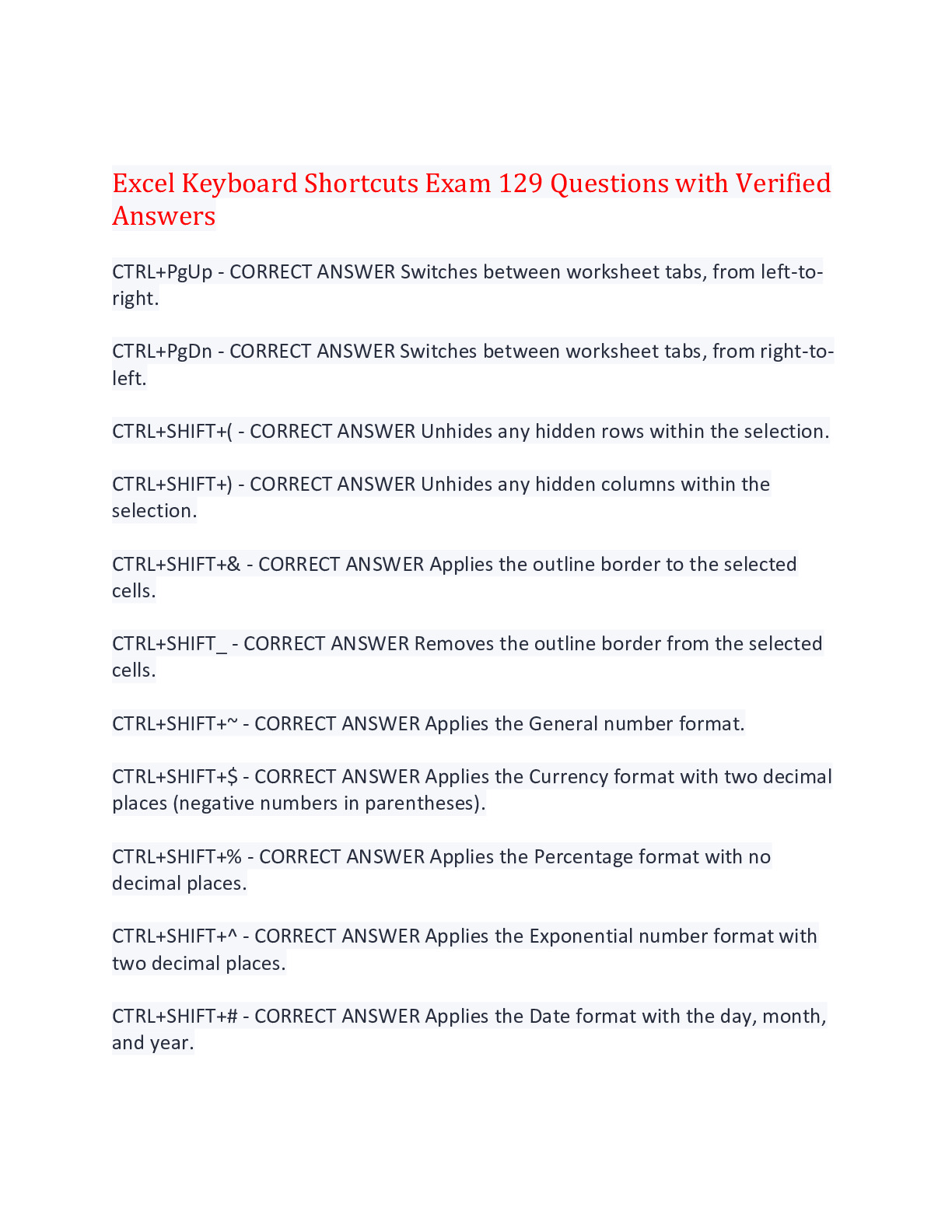
Excel Keyboard Shortcuts Exam 129 Questions with Verified Answers,100% CORRECT
Excel Keyboard Shortcuts Exam 129 Questions with Verified Answers CTRL+PgUp - CORRECT ANSWER Switches between worksheet tabs, from left-to-right. CTR... [Show More] L+PgDn - CORRECT ANSWER Switches between worksheet tabs, from right-to-left. CTRL+SHIFT+( - CORRECT ANSWER Unhides any hidden rows within the selection. CTRL+SHIFT+) - CORRECT ANSWER Unhides any hidden columns within the selection. CTRL+SHIFT+& - CORRECT ANSWER Applies the outline border to the selected cells. CTRL+SHIFT_ - CORRECT ANSWER Removes the outline border from the selected cells. CTRL+SHIFT+~ - CORRECT ANSWER Applies the General number format. CTRL+SHIFT+$ - CORRECT ANSWER Applies the Currency format with two decimal places (negative numbers in parentheses). CTRL+SHIFT+% - CORRECT ANSWER Applies the Percentage format with no decimal places. CTRL+SHIFT+^ - CORRECT ANSWER Applies the Exponential number format with two decimal places. CTRL+SHIFT+# - CORRECT ANSWER Applies the Date format with the day, month, and year. CTRL+SHIFT+@ - CORRECT ANSWER Applies the Time format with the hour and minute, and AM or PM. CTRL+SHIFT+! - CORRECT ANSWER Applies the Number format with two decimal places, thousands separator, and minus sign (-) for negative values. CTRL+SHIFT+* - CORRECT ANSWER Selects the current region around the active cell (the data area enclosed by blank rows and blank columns). In a PivotTable, it selects the entire PivotTable report. CTRL+SHIFT+: - CORRECT ANSWER Enters the current time. CTRL+SHIFT+" - CORRECT ANSWER Copies the value from the cell above the active cell into the cell or the Formula Bar. CTRL+SHIFT+Plus (+) - CORRECT ANSWER Displays the Insert dialog box to insert blank cells. CTRL+Minus (-) - CORRECT ANSWER Displays the Delete dialog box to delete the selected cells. CTRL+; - CORRECT ANSWER Enters the current date. CTRL+` - CORRECT ANSWER Alternates between displaying cell values and displaying formulas in the worksheet. CTRL+' - CORRECT ANSWER Copies a formula from the cell above the active cell into the cell or the Formula Bar. CTRL+1 - CORRECT ANSWER Displays the Format Cells dialog box. CTRL+2 - CORRECT ANSWER Applies or removes bold formatting. CTRL+3 - CORRECT ANSWER Applies or removes italic formatting. CTRL+4 - CORRECT ANSWER Applies or removes underlining. CTRL+5 - CORRECT ANSWER Applies or removes strikethrough. CTRL+6 - CORRECT ANSWER Alternates between hiding objects, displaying objects, and displaying placeholders for objects. CTRL+8 - CORRECT ANSWER Displays or hides the outline symbols. CTRL+9 - CORRECT ANSWER Hides the selected rows. CTRL+0 - CORRECT ANSWER Hides the selected columns. CTRL+A - CORRECT ANSWER Selects the entire worksheet. If the worksheet contains data, CTRL+A selects the current region. Pressing CTRL+A a second time selects the current region and its summary rows. Pressing CTRL+A a third time selects the entire worksheet. When the insertion point is to the right of a function name in a formula, displays the Function Arguments dialog box. CTRL+SHIFT+A - CORRECT ANSWER Inserts the argument names and parentheses when the insertion point is to the right of a function name in a formula. CTRL+B - CORRECT ANSWER Applies or removes bold formatting. CTRL+C - CORRECT ANSWER Copies the selected cells. CTRL+C followed by another CTRL+C displays the Clipboard. CTRL+D - CORRECT ANSWER Uses the Fill Down command to copy the contents and format of the topmost cell of a selected range into the cells below. CTRL+E - CORRECT ANSWER Available. CTRL+F - CORRECT ANSWER Displays the Find and Replace dialog box, with the Find tab selected. Same as SHIFT+F5. SHIFT+F5 - CORRECT ANSWER Displays the Find and Replace dialog box, with the Find tab selected. Same as CTRL+F. SHIFT+F4 - CORRECT ANSWER Repeats the last Find action. CTRL+SHIFT+F - CORRECT ANSWER Opens the Format Cells dialog box with the Font tab selected. Same as CTRL+SHIFT+P. CTRL+G - CORRECT ANSWER Displays the Go To dialog box. Same as F5. CTRL+H - CORRECT ANSWER Displays the Find and Replace dialog box, with the Replace tab selected. CTRL+I - CORRECT ANSWER Applies or removes italic formatting. CTRL+J - CORRECT ANSWER Available. CTRL+K - CORRECT ANSWER Displays the Insert Hyperlink dialog box for new hyperlinks or the Edit Hyperlink dialog box for selected existing hyperlinks. CTRL+L - CORRECT ANSWER Available. CTRL+M - CORRECT ANSWER Available. CTRL+N - CORRECT ANSWER Creates a new, blank workbook. CTRL+O - CORRECT ANSWER Displays the Open dialog box to open or find a file. CTRL+SHIFT+O - CORRECT ANSWER Selects all cells that contain comments. CTRL+P - CORRECT ANSWER Displays the Print dialog box. CTRL+SHIFT+P - CORRECT ANSWER Opens the Format Cells dialog box with the Font tab selected. Same as CTRL+SHIFT+F. CTRL+Q - CORRECT ANSWER Available. CTRL+R - CORRECT ANSWER Uses the Fill Right command to copy the contents and format of the leftmost cell of a selected range into the cells to the right. CTRL+S - CORRECT ANSWER Saves the active file with its current file name, location, and file format. CTRL+T - CORRECT ANSWER Displays the Create Table dialog box. CTRL+U - CORRECT ANSWER Applies or removes underlining. CTRL+SHIFT+U - CORRECT ANSWER Switches between expanding and collapsing of the formula bar. CTRL+V - CORRECT ANSWER Inserts the contents of the Clipboard at the insertion point and replaces any selection. Available only after you have cut or copied an object, text, or cell contents. CTRL+ALT+V - CORRECT ANSWER Displays the Paste Special dialog box. Available only after you have cut or copied an object, text, or cell contents on a worksheet or in another program. CTRL+W - CORRECT ANSWER Closes the selected workbook window. CTRL+X - CORRECT ANSWER Cuts the selected cells. CTRL+Y - CORRECT ANSWER Repeats the last command or action, if possible. CTRL+Z - CORRECT ANSWER Uses the Undo command to reverse the last command or to delete the last entry that you typed. CTRL+SHIFT+Z - CORRECT ANSWER Uses the Undo or Redo command to reverse or restore the last automatic correction when AutoCorrect Smart Tags are displayed. F1 - CORRECT ANSWER Displays the Microsoft Office Excel Help task pane. CTRL+F1 - CORRECT ANSWER Displays or hides the Ribbon, a component of the Microsoft Office Fluent user interface. ALT+F1 - CORRECT ANSWER Creates a chart of the data in the current range. ALT+SHIFT+F1 - CORRECT ANSWER Inserts a new worksheet. F2 - CORRECT ANSWER Edits the active cell and positions the insertion point at the end of the cell contents. It also moves the insertion point into the Formula Bar when editing in a cell is turned off. SHIFT+F2 - CORRECT ANSWER Adds or edits a cell comment. CTRL+F2 - CORRECT ANSWER Displays the Print Preview window. F3 - CORRECT ANSWER Displays the Paste Name dialog box. SHIFT+F3 - CORRECT ANSWER Displays the Insert Function dialog box. F4 - CORRECT ANSWER Repeats the last command or action, if possible. When a cell reference or range is selected in a formula, F4 cycles through the various combinations of absolute and relative references. CTRL+F4 - CORRECT ANSWER Closes the selected workbook window. F5 - CORRECT ANSWER Displays the Go To dialog box. Same as CTRL+G. CTRL+F5 - CORRECT ANSWER Restores the window size of the selected workbook window. F6 - CORRECT ANSWER Switches between the worksheet, Ribbon, task pane, and Zoom controls. In a worksheet that has been split (View menu, Manage This Window, Freeze Panes, Split Window command), F6 includes the split panes when switching between panes and the Ribbon area. SHIFT+F6 - CORRECT ANSWER Switches between the worksheet, Zoom controls, task pane, and Ribbon. CTRL+F6 - CORRECT ANSWER Switches to the next workbook window when more than one workbook window is open. F7 - CORRECT ANSWER Displays the Spelling dialog box to check spelling in the active worksheet or selected range. CTRL+F7 - CORRECT ANSWER Performs the Move command on the workbook window when it is not maximized. Use the arrow keys to move the window, and when finished press ENTER, or ESC to cancel. F8 - CORRECT ANSWER Turns extend mode on or off. In extend mode, Extended Selection appears in the status line, and the arrow keys extend the selection. SHIFT+F8 - CORRECT ANSWER Enables you to add a nonadjacent cell or range to a selection of cells by using the arrow keys. CTRL+F8 - CORRECT ANSWER Performs the Size command (on the Control menu for the workbook window) when a workbook is not maximized. ALT+F8 - CORRECT ANSWER Displays the Macro dialog box to create, run, edit, or delete a macro. F9 - CORRECT ANSWER Calculates all worksheets in all open workbooks. SHIFT+F9 - CORRECT ANSWER Calculates the active worksheet. CTRL+ALT+F9 - CORRECT ANSWER Calculates all worksheets in all open workbooks, regardless of whether they have changed since the last calculation. CTRL+ALT+SHIFT+F9 - CORRECT ANSWER Rechecks dependent formulas, and then calculates all cells in all open workbooks, including cells not marked as needing to be calculated. CTRL+F9 - CORRECT ANSWER Minimizes a workbook window to an icon. F10 - CORRECT ANSWER Turns key tips on or off. SHIFT+F10 - CORRECT ANSWER Displays the shortcut menu for a selected item. ALT+SHIFT+F10 - CORRECT ANSWER Displays the menu or message for a smart tag. If more than one smart tag is present, it switches to the next smart tag and displays its menu or message. CTRL+F10 - CORRECT ANSWER Maximizes or restores the selected workbook window. F11 - CORRECT ANSWER Creates a chart of the data in the current range. SHIFT+F11 - CORRECT ANSWER Inserts a new worksheet. ALT+F11 - CORRECT ANSWER Opens the Microsoft Visual Basic Editor, in which you can create a macro by using Visual Basic for Applications (VBA). F12 - CORRECT ANSWER Displays the Save As dialog box. CTRL+ARROW KEY - CORRECT ANSWER Moves to the edge of the current data region in a worksheet. SHIFT+ARROW KEY - CORRECT ANSWER Extends the selection of cells by one cell. CTRL+SHIFT+ARROW KEY - CORRECT ANSWER Extends the selection of cells to the last nonblank cell in the same column or row as the active cell, or if the next cell is blank, extends the selection to the next nonblank cell. DOWN ARROW - CORRECT ANSWER Opens a selected drop-down list (or ALT+DOWN ARROW). END - CORRECT ANSWER Moves to the cell in the lower-right corner of the window when SCROLL LOCK is turned on. Also selects the last command on the menu when a menu or submenu is visible. CTRL+END - CORRECT ANSWER Moves to the last cell on a worksheet, in the lowest used row of the rightmost used column. If the cursor is in the formula bar, CTRL+END moves the cursor to the end of the text. CTRL+SHIFT+END - CORRECT ANSWER Extends the selection of cells to the last used cell on the worksheet (lower-right corner). If the cursor is in the formula bar, CTRL+SHIFT+END selects all text in the formula bar from the cursor position to the end—this does not affect the height of the formula bar. ALT+ENTER - CORRECT ANSWER Starts a new line in the same cell. CTRL+ENTER - CORRECT ANSWER Fills the selected cell range with the current entry. SHIFT+ENTER - CORRECT ANSWER Completes a cell entry and selects the cell above. HOME - CORRECT ANSWER Moves to the beginning of a row in a worksheet. Moves to the cell in the upper-left corner of the window when SCROLL LOCK is turned on. Selects the first command on the menu when a menu or submenu is visible. CTRL+HOME - CORRECT ANSWER Moves to the beginning of a worksheet. CTRL+SHIFT+HOME - CORRECT ANSWER Extends the selection of cells to the beginning of the worksheet. PAGE DOWN - CORRECT ANSWER Moves one screen down in a worksheet. ALT+PAGE DOWN - CORRECT ANSWER Moves one screen to the right in a worksheet. CTRL+PAGE DOWN - CORRECT ANSWER Moves to the next sheet in a workbook. CTRL+SHIFT+PAGE DOWN - CORRECT ANSWER Selects the current and next sheet in a workbook. PAGE UP - CORRECT ANSWER Moves one screen up in a worksheet. ALT+PAGE UP - CORRECT ANSWER Moves one screen to the left in a worksheet. CTRL+PAGE UP - CORRECT ANSWER Moves to the previous sheet in a workbook. CTRL+SHIFT+PAGE UP - CORRECT ANSWER Selects the current and previous sheet in a workbook. SPACEBAR - CORRECT ANSWER In a dialog box, performs the action for the selected button, or selects or clears a check box. CTRL+SPACEBAR - CORRECT ANSWER Selects an entire column in a worksheet. SHIFT+SPACEBAR - CORRECT ANSWER Selects an entire row in a worksheet. CTRL+SHIFT+SPACEBAR - CORRECT ANSWER Selects the entire worksheet. If the worksheet contains data, CTRL+SHIFT+SPACEBAR selects the current region. Pressing CTRL+SHIFT+SPACEBAR a second time selects the current region and its summary rows. Pressing CTRL+SHIFT+SPACEBAR a third time selects the entire worksheet. When an object is selected, CTRL+SHIFT+SPACEBAR selects all objects on a worksheet. ALT+SPACEBAR - CORRECT ANSWER Displays the Control menu for the Microsoft Office Excel window. SHIFT+TAB - CORRECT ANSWER Moves to the previous cell in a worksheet or the previous option in a dialog box. CTRL+TAB - CORRECT ANSWER Switches to the next tab in dialog box. CTRL+SHIFT+TAB - CORRECT ANSWER Switches to the previous tab in a dialog box. [Show Less]
- Exam
- $11.45
- 0
- 46

Excel Module 2 SAM Training Exam 23 Questions with Verified Answers,100% CORRECT
Excel Module 2 SAM Training Exam 23 Questions with Verified Answers Wrap the text in cell A6 so that all the text is visible in the cell. - CORRECT ANSW... [Show More] ER Click cell A6. In the Alignment group, click the wrao text button. Use Flash Fill to fill range E4:E15 after typing "[email protected]" in cell E4 and "Sal" in cell E5 - CORRECT ANSWER Click cell E4. Type "[email protected]" in cell E4, and press Enter. Type "Sal" in cell E5, and press enter. Enter a formula using arithmetic operators and parentheses in cell B14 that adds the monthly expenses in cells B9, B10, and B11, and then multiplies that result by 12. - CORRECT ANSWER Select cell B14. Type "=(" in cell B14. Click cell B9. Type + in b14. Click b10. Type + in cell b14. Click b11. Type ) in b14. Type *12 in b14. On the formula bar, click the enter button. In cell B19, create a formula by entering cell references that subtracts can B6 from B5, and then subtracts cell B18. - CORRECT ANSWER Click cell b19. Type = to begin formula. Click b5. Type - in b19. Click b6. Type - in b19. Click b18. Press enter. In cell D19, create a formula using the COUNT function to count the number of values in the range d5:d18. - CORRECT ANSWER Select d19. Type =COUNT(. Select d5-d18. Type ). Press enter. In cell F19, Create a formula using the COUNTA function that counts the number of cells that are not empty in the range F5:F18. - CORRECT ANSWER Click cell f19. Click the formulas tab. Click the more functions button. Point to statistical. Click COUNTA. Type f5:f18 in the Value1 box. Click Ok. For range B4:B15, create a New conditional formatting rule that formats the top five values in the range with a Blue, Accent 5 cell background color. - CORRECT ANSWER Click and drag to select cells B4:B15. In the styles group, click the conditional formatting button. Click new rule. In the select rule type section, click format only top or bottom ranked values. Select the value box, which currently displays the number 10, type 5. Click format. Click the fill tab. In the background colors section, click the blue, accent 5 option. Click ok. Click ok. Apply the Berlin theme to the current workbook. - CORRECT ANSWER Click the page layout ribbon. Click the themes button. Click the Berlin option. change the fill color of cell d9 to blue, accent 1, lighter 60% (theme colors section, row 3, column 5). - CORRECT ANSWER Select D9. In the Font group, click the fill color arrow. Choose the color needed. apply thick outside borders to the range A8:D8. - CORRECT ANSWER Select A8-D8. In the Font group click the borders arrow. Click the thick outside borders option. Click cell D10. Add an outline border with a blue accent five line color to sell D19 then select A3. - CORRECT ANSWER Select D19. In the font group on the home tab click on the borders arrow. Click more borders. In the line section click the color arrow. Click blue accent 5. In the presets section of the dialog box, click the outline button. Click ok. Click A3. Apply the 03/14/12 Date number format to cell D4. - CORRECT ANSWER Select D4. In the number group on the ribbon click the dialog box launcher. In the type list, click 03/14/12 to select a new date number format. Click ok. For values in the range B3:B12, adjust the number of decimal places so that two decimal places are displayed. - CORRECT ANSWER Select cells B3:B12. In the number group click the increase decimal button. Click it again. Apply the percent Number Format, with no decimal places, to the range C4:C15. - CORRECT ANSWER Select C4:C15. In the number group click the percent style button. Edit the conditional formatting rule for range for range B5:B16 to highlight cells whose value is less than $25,000. Use the same cell formatting as in the original rule - CORRECT ANSWER Select B5:B16. In the styles group click the conditional formatting button. Click manage rules. Click edit rule. In the edit formatting dialog box under format only cells with click the greater than arrow. Click less than. Click ok. Click ok. Clear the conditional formatting rule from the range B4:B15. - CORRECT ANSWER Select B4:B15. I am at the styles group click the conditional formatting button. Click clear rules. Click clear rules from selected cells. Hide column F. - CORRECT ANSWER 1. Click the column heading for column F 2. In the Cells group, click the Format button 3. Point to Hide and Unhide 4. Click Hide Columns Change the height of row 2 to approximately 27 points. - CORRECT ANSWER Click cell A2. Click 2 and drag down to 27 points. Check spelling in the entire worksheet, accepting the suggested correction. - CORRECT ANSWER Click the review tab. Click the spelling button. Click change. Click yes. Click ok. Print 3 copies of the Sales Forecast Worksheet. - CORRECT ANSWER Click the file tab. Click print. Click the copies text box and type 3. Click the print button. Change the worksheet margins to the narrow margin style. - CORRECT ANSWER Click the page layout tab. Click the margins button. Click narrow. Add the text Confidential to the center header section, and then click cell A4 to deselect the header. - CORRECT ANSWER Click the view tab. Click the page layout button. Click the center section of the header placeholder, which contains the text "Add header". Type Confidential in the center header. In the worksheet, click cell A4. Highlight cells in the range B4:B15 whose value is less than $50000 using Yellow Fill with Dark Yellow Text. - CORRECT ANSWER Select B4:B15. Click Conditional Formatting button. Point to Highlight Cells Rules. Click Less Than. Type 50000. Click the format cells arrow. Click the yellow fill with dark yellow text option. Click ok. [Show Less]
- Exam
- $9.95
- 0
- 44

Excel Keyboard Shortcuts Exam 136 Questions with Verified Answers,100% CORRECT
Excel Keyboard Shortcuts Exam 136 Questions with Verified Answers CTRL+PgUp - CORRECT ANSWER Switches between worksheet tabs, from left-to-right. CTR... [Show More] L+PgDn - CORRECT ANSWER Switches between worksheet tabs, from right-to-left. CTRL+SHIFT+( - CORRECT ANSWER Unhides any hidden rows within the selection. CTRL+SHIFT+) - CORRECT ANSWER Unhides any hidden columns within the selection. CTRL+SHIFT+& - CORRECT ANSWER Applies the outline border to the selected cells. CTRL+SHIFT_ - CORRECT ANSWER Removes the outline border from the selected cells. CTRL+SHIFT+~ - CORRECT ANSWER Applies the General number format. CTRL+SHIFT+$ - CORRECT ANSWER Applies the Currency format with two decimal places (negative numbers in parentheses). CTRL+SHIFT+% - CORRECT ANSWER Applies the Percentage format with no decimal places. CTRL+SHIFT+^ - CORRECT ANSWER Applies the Exponential number format with two decimal places. CTRL+SHIFT+# - CORRECT ANSWER Applies the Date format with the day, month, and year. CTRL+SHIFT+@ - CORRECT ANSWER Applies the Time format with the hour and minute, and AM or PM. CTRL+SHIFT+! - CORRECT ANSWER Applies the Number format with two decimal places, thousands separator, and minus sign (-) for negative values. CTRL+SHIFT+* - CORRECT ANSWER Selects the current region around the active cell (the data area enclosed by blank rows and blank columns). In a PivotTable, it selects the entire PivotTable report. CTRL+SHIFT+: - CORRECT ANSWER Enters the current time. CTRL+SHIFT+" - CORRECT ANSWER Copies the value from the cell above the active cell into the cell or the Formula Bar. CTRL+SHIFT+Plus (+) - CORRECT ANSWER Displays the Insert dialog box to insert blank cells. CTRL+Minus (-) - CORRECT ANSWER Displays the Delete dialog box to delete the selected cells. CTRL+; - CORRECT ANSWER Enters the current date. CTRL+` - CORRECT ANSWER Alternates between displaying cell values and displaying formulas in the worksheet. CTRL+' - CORRECT ANSWER Copies a formula from the cell above the active cell into the cell or the Formula Bar. CTRL+1 - CORRECT ANSWER Displays the Format Cells dialog box. CTRL+2 - CORRECT ANSWER Applies or removes bold formatting. CTRL+3 - CORRECT ANSWER Applies or removes italic formatting. CTRL+4 - CORRECT ANSWER Applies or removes underlining. CTRL+5 - CORRECT ANSWER Applies or removes strikethrough. CTRL+6 - CORRECT ANSWER Alternates between hiding objects, displaying objects, and displaying placeholders for objects. CTRL+8 - CORRECT ANSWER Displays or hides the outline symbols. CTRL+9 - CORRECT ANSWER Hides the selected rows. CTRL+0 - CORRECT ANSWER Hides the selected columns. CTRL+A - CORRECT ANSWER Selects the entire worksheet. If the worksheet contains data, CTRL+A selects the current region. Pressing CTRL+A a second time selects the current region and its summary rows. Pressing CTRL+A a third time selects the entire worksheet. When the insertion point is to the right of a function name in a formula, displays the Function Arguments dialog box. CTRL+SHIFT+A - CORRECT ANSWER Inserts the argument names and parentheses when the insertion point is to the right of a function name in a formula. CTRL+B - CORRECT ANSWER Applies or removes bold formatting. CTRL+C - CORRECT ANSWER Copies the selected cells. CTRL+C followed by another CTRL+C displays the Clipboard. CTRL+D - CORRECT ANSWER Uses the Fill Down command to copy the contents and format of the topmost cell of a selected range into the cells below. CTRL+E - CORRECT ANSWER Available. CTRL+F - CORRECT ANSWER Displays the Find and Replace dialog box, with the Find tab selected. Same as SHIFT+F5. SHIFT+F5 - CORRECT ANSWER Displays the Find and Replace dialog box, with the Find tab selected. Same as CTRL+F. SHIFT+F4 - CORRECT ANSWER Repeats the last Find action. CTRL+SHIFT+F - CORRECT ANSWER Opens the Format Cells dialog box with the Font tab selected. Same as CTRL+SHIFT+P. CTRL+G - CORRECT ANSWER Displays the Go To dialog box. Same as F5. CTRL+H - CORRECT ANSWER Displays the Find and Replace dialog box, with the Replace tab selected. CTRL+I - CORRECT ANSWER Applies or removes italic formatting. CTRL+J - CORRECT ANSWER Available. CTRL+K - CORRECT ANSWER Displays the Insert Hyperlink dialog box for new hyperlinks or the Edit Hyperlink dialog box for selected existing hyperlinks. CTRL+L - CORRECT ANSWER Available. CTRL+M - CORRECT ANSWER Available. CTRL+N - CORRECT ANSWER Creates a new, blank workbook. CTRL+O - CORRECT ANSWER Displays the Open dialog box to open or find a file. CTRL+SHIFT+O - CORRECT ANSWER Selects all cells that contain comments. CTRL+P - CORRECT ANSWER Displays the Print dialog box. CTRL+SHIFT+P - CORRECT ANSWER Opens the Format Cells dialog box with the Font tab selected. Same as CTRL+SHIFT+F. CTRL+Q - CORRECT ANSWER Available. CTRL+R - CORRECT ANSWER Uses the Fill Right command to copy the contents and format of the leftmost cell of a selected range into the cells to the right. CTRL+S - CORRECT ANSWER Saves the active file with its current file name, location, and file format. CTRL+T - CORRECT ANSWER Displays the Create Table dialog box. CTRL+U - CORRECT ANSWER Applies or removes underlining. CTRL+SHIFT+U - CORRECT ANSWER Switches between expanding and collapsing of the formula bar. CTRL+V - CORRECT ANSWER Inserts the contents of the Clipboard at the insertion point and replaces any selection. Available only after you have cut or copied an object, text, or cell contents. CTRL+ALT+V - CORRECT ANSWER Displays the Paste Special dialog box. Available only after you have cut or copied an object, text, or cell contents on a worksheet or in another program. CTRL+W - CORRECT ANSWER Closes the selected workbook window. CTRL+X - CORRECT ANSWER Cuts the selected cells. CTRL+Y - CORRECT ANSWER Repeats the last command or action, if possible. CTRL+Z - CORRECT ANSWER Uses the Undo command to reverse the last command or to delete the last entry that you typed. CTRL+SHIFT+Z - CORRECT ANSWER Uses the Undo or Redo command to reverse or restore the last automatic correction when AutoCorrect Smart Tags are displayed. F1 - CORRECT ANSWER Displays the Microsoft Office Excel Help task pane. CTRL+F1 - CORRECT ANSWER Displays or hides the Ribbon, a component of the Microsoft Office Fluent user interface. ALT+F1 - CORRECT ANSWER Creates a chart of the data in the current range. ALT+SHIFT+F1 - CORRECT ANSWER Inserts a new worksheet. F2 - CORRECT ANSWER Edits the active cell and positions the insertion point at the end of the cell contents. It also moves the insertion point into the Formula Bar when editing in a cell is turned off. SHIFT+F2 - CORRECT ANSWER Adds or edits a cell comment. CTRL+F2 - CORRECT ANSWER Displays the Print Preview window. F3 - CORRECT ANSWER Displays the Paste Name dialog box. SHIFT+F3 - CORRECT ANSWER Displays the Insert Function dialog box. F4 - CORRECT ANSWER Repeats the last command or action, if possible. When a cell reference or range is selected in a formula, F4 cycles through the various combinations of absolute and relative references. CTRL+F4 - CORRECT ANSWER Closes the selected workbook window. F5 - CORRECT ANSWER Displays the Go To dialog box. Same as CTRL+G. CTRL+F5 - CORRECT ANSWER Restores the window size of the selected workbook window. F6 - CORRECT ANSWER Switches between the worksheet, Ribbon, task pane, and Zoom controls. In a worksheet that has been split (View menu, Manage This Window, Freeze Panes, Split Window command), F6 includes the split panes when switching between panes and the Ribbon area. SHIFT+F6 - CORRECT ANSWER Switches between the worksheet, Zoom controls, task pane, and Ribbon. CTRL+F6 - CORRECT ANSWER Switches to the next workbook window when more than one workbook window is open. F7 - CORRECT ANSWER Displays the Spelling dialog box to check spelling in the active worksheet or selected range. CTRL+F7 - CORRECT ANSWER Performs the Move command on the workbook window when it is not maximized. Use the arrow keys to move the window, and when finished press ENTER, or ESC to cancel. F8 - CORRECT ANSWER Turns extend mode on or off. In extend mode, Extended Selection appears in the status line, and the arrow keys extend the selection. SHIFT+F8 - CORRECT ANSWER Enables you to add a nonadjacent cell or range to a selection of cells by using the arrow keys. CTRL+F8 - CORRECT ANSWER Performs the Size command (on the Control menu for the workbook window) when a workbook is not maximized. ALT+F8 - CORRECT ANSWER Displays the Macro dialog box to create, run, edit, or delete a macro. F9 - CORRECT ANSWER Calculates all worksheets in all open workbooks. SHIFT+F9 - CORRECT ANSWER Calculates the active worksheet. CTRL+ALT+F9 - CORRECT ANSWER Calculates all worksheets in all open workbooks, regardless of whether they have changed since the last calculation. CTRL+ALT+SHIFT+F9 - CORRECT ANSWER Rechecks dependent formulas, and then calculates all cells in all open workbooks, including cells not marked as needing to be calculated. CTRL+F9 - CORRECT ANSWER Minimizes a workbook window to an icon. F10 - CORRECT ANSWER Turns key tips on or off. SHIFT+F10 - CORRECT ANSWER Displays the shortcut menu for a selected item. ALT+SHIFT+F10 - CORRECT ANSWER Displays the menu or message for a smart tag. If more than one smart tag is present, it switches to the next smart tag and displays its menu or message. CTRL+F10 - CORRECT ANSWER Maximizes or restores the selected workbook window. F11 - CORRECT ANSWER Creates a chart of the data in the current range. SHIFT+F11 - CORRECT ANSWER Inserts a new worksheet. ALT+F11 - CORRECT ANSWER Opens the Microsoft Visual Basic Editor, in which you can create a macro by using Visual Basic for Applications (VBA). F12 - CORRECT ANSWER Displays the Save As dialog box. CTRL+ARROW KEY - CORRECT ANSWER Moves to the edge of the current data region in a worksheet. SHIFT+ARROW KEY - CORRECT ANSWER Extends the selection of cells by one cell. CTRL+SHIFT+ARROW KEY - CORRECT ANSWER Extends the selection of cells to the last nonblank cell in the same column or row as the active cell, or if the next cell is blank, extends the selection to the next nonblank cell. DOWN ARROW - CORRECT ANSWER Opens a selected drop-down list (or ALT+DOWN ARROW). END - CORRECT ANSWER Moves to the cell in the lower-right corner of the window when SCROLL LOCK is turned on. Also selects the last command on the menu when a menu or submenu is visible. CTRL+END - CORRECT ANSWER Moves to the last cell on a worksheet, in the lowest used row of the rightmost used column. If the cursor is in the formula bar, CTRL+END moves the cursor to the end of the text. CTRL+SHIFT+END - CORRECT ANSWER Extends the selection of cells to the last used cell on the worksheet (lower-right corner). If the cursor is in the formula bar, CTRL+SHIFT+END selects all text in the formula bar from the cursor position to the end—this does not affect the height of the formula bar. ALT+ENTER - CORRECT ANSWER Starts a new line in the same cell. CTRL+ENTER - CORRECT ANSWER Fills the selected cell range with the current entry. SHIFT+ENTER - CORRECT ANSWER Completes a cell entry and selects the cell above. HOME - CORRECT ANSWER Moves to the beginning of a row in a worksheet. Moves to the cell in the upper-left corner of the window when SCROLL LOCK is turned on. Selects the first command on the menu when a menu or submenu is visible. CTRL+HOME - CORRECT ANSWER Moves to the beginning of a worksheet. CTRL+SHIFT+HOME - CORRECT ANSWER Extends the selection of cells to the beginning of the worksheet. PAGE DOWN - CORRECT ANSWER Moves one screen down in a worksheet. ALT+PAGE DOWN - CORRECT ANSWER Moves one screen to the right in a worksheet. CTRL+PAGE DOWN - CORRECT ANSWER Moves to the next sheet in a workbook. CTRL+SHIFT+PAGE DOWN - CORRECT ANSWER Selects the current and next sheet in a workbook. PAGE UP - CORRECT ANSWER Moves one screen up in a worksheet. ALT+PAGE UP - CORRECT ANSWER Moves one screen to the left in a worksheet. CTRL+PAGE UP - CORRECT ANSWER Moves to the previous sheet in a workbook. CTRL+SHIFT+PAGE UP - CORRECT ANSWER Selects the current and previous sheet in a workbook. SPACEBAR - CORRECT ANSWER In a dialog box, performs the action for the selected button, or selects or clears a check box. CTRL+SPACEBAR - CORRECT ANSWER Selects an entire column in a worksheet. SHIFT+SPACEBAR - CORRECT ANSWER Selects an entire row in a worksheet. CTRL+SHIFT+SPACEBAR - CORRECT ANSWER Selects the entire worksheet. If the worksheet contains data, CTRL+SHIFT+SPACEBAR selects the current region. Pressing CTRL+SHIFT+SPACEBAR a second time selects the current region and its summary rows. Pressing CTRL+SHIFT+SPACEBAR a third time selects the entire worksheet. When an object is selected, CTRL+SHIFT+SPACEBAR selects all objects on a worksheet. ALT+SPACEBAR - CORRECT ANSWER Displays the Control menu for the Microsoft Office Excel window. SHIFT+TAB - CORRECT ANSWER Moves to the previous cell in a worksheet or the previous option in a dialog box. CTRL+TAB - CORRECT ANSWER Switches to the next tab in dialog box. CTRL+SHIFT+TAB - CORRECT ANSWER Switches to the previous tab in a dialog box. Find and Replace - CORRECT ANSWER CTRL + H Formatting a cell to "fit" - CORRECT ANSWER ALT + HOI Enter a cell - CORRECT ANSWER F2 Bold a cell - CORRECT ANSWER CTRL + B Undo - CORRECT ANSWER CTRL + Z Highlight a row - CORRECT ANSWER SHIFT + Spacebar Highlight a column - CORRECT ANSWER CTRL + Spacebar [Show Less]
- Exam
- $11.45
- 0
- 36

Go Skills Microsoft Excel Basic and Advanced Exam 169 Questions with Verified Answers,100% CORRECT
Go Skills Microsoft Excel Basic and Advanced Exam 169 Questions with Verified Answers A portion of Excel's user interface has been circled in the imag... [Show More] e below. What is the name of that area? - CORRECT ANSWER The Quick Access Toolbar (QAT) A portion of Excel's user interface has been circled below. What is the name of that area? - CORRECT ANSWER The Font Group What has been circled in the image below? - CORRECT ANSWER Ribbon Tabs How would we refer to the cell indicated in the image below? - CORRECT ANSWER C7 What value is contained in cell B8? - CORRECT ANSWER 65 Which user interface element is indicated by the red arrow? - CORRECT ANSWER Horizontal Scroll Bar Assume that you enter data in cell A6 and press Tab, then enter data in cell B6 and press Tab, then enter data in cell C6 and press Enter. Which cell will you find yourself in? - CORRECT ANSWER A7 What does the command shown below actually do? - CORRECT ANSWER Undoes previous actions What would be the easiest way to select cells A5, B5 and C5? - CORRECT ANSWER Use the mouse, select A5, hold down the left mouse button and drag over to C5 In order to enter data into a cell you must: - CORRECT ANSWER Have the cell selected, then start typing If column B is too narrow to show all the text you've typed into a cell, how could you expand it to display the text? - CORRECT ANSWER Move your mouse between the column B and column C headers, then drag the column wider There are 3 areas marked in the image below. Assuming that you were trying to locate a file that you worked on several months ago, which area would you want to explore? - CORRECT ANSWER 2 If you wanted to customize your formatting to a high degree, where would you find the largest collection of formatting tools? - CORRECT ANSWER The Format Cells dialog box If your cursor is in the middle of the worksheet, what is the fastest way to call up this dialog box? - CORRECT ANSWER Right click on a cell, choose Format Cells, and click Border If you wanted to format numeric values with a less common foreign currency symbol, what would you have to do? - CORRECT ANSWER Go to the Format Cells dialog and change the symbol in the currency or accounting number formats Given the picture below, what would we want to enter in cell D5 to get the product of B5 and C5? - CORRECT ANSWER =B5*C5 Given the image below, what is the best way to get B10 to show the sum of the values from B5 through B9? - CORRECT ANSWER Select B10, go to the Home Tab and click the AutoSum button on the Editing group Given the image below, what would you expect to happen if you selected C10, then went to the Home tab, selected AutoSum from the Editing group, and chose Average from the list? - CORRECT ANSWER A formula would be entered in C10 that averaged the values of cells C5 through C9 Assuming you typed the following in the formula bar, what would be returned to the cell when you hit Enter? - CORRECT ANSWER B2+C2 What formula would return the product of 6 x 4 for the Apples row? - CORRECT ANSWER =B3*C3 Which formula would you use to divide Total Sales by the number of Days for Oranges? - CORRECT ANSWER =B2/C2 If B5 contains the formula =$A$1+B1, what would the formula read if copied to B6? - CORRECT ANSWER =$A$1+B2 Which method for copying cells results in just the formulas being copied? - CORRECT ANSWER Copying formulas, then choosing PasteSpecial and clicking Formulas Suppose you select cells B4:C5, and then enter =B$3+20 and press CTRL + Enter. What will C5 contain? - CORRECT ANSWER =C$3+20 Demonstrate that you can apply the concepts from this video to other Excel functions. How many parameters are required for the PV function? - CORRECT ANSWER 3 Demonstrate that you can apply the concepts from this video to other Excel functions. Assuming we clicked C5 at this point in our formula, which parameter would it be used for? - CORRECT ANSWER kpi_name Demonstrate that you can apply the concepts from this video to other Excel functions. What is missing in the following? - CORRECT ANSWER A closing parenthesis Which is the best formula to add cells A1 and A4:A6 (A4 through A6) together? - CORRECT ANSWER =SUM(A1,A4:A6) There is data in the cells B4:B15, with the following formula used to subtotal the data in B9: =SUBTOTAL(9,B5:B8). Which would be best formula to ensure that we've summed up all values from B4 through B15? - CORRECT ANSWER =SUBTOTAL(9,B4:B15) A5 shows a value of 1234.56. Which of the following methods would you use to round the value 1235? - CORRECT ANSWER =ROUND(A5,0) Which formula counts the number of non-blank items in the cells A1:A10 (A1 through A10)? - CORRECT ANSWER =COUNTA(A1:A10) Which function returns the most frequently occurring number in a data set? - CORRECT ANSWER MODE() Which formula returns the arithmetic mean of the numbers in a data set? - CORRECT ANSWER =AVERAGE(A1:A10) Which formula is guaranteed to return the phrase "You win!" if the value in cell B6 is 29? - CORRECT ANSWER =IF(OR(B6=29,C6=10),"You win!","Try again!") Which is the best formula to return the phrase "You win!" if both cell B6 equals 29 and cell C6 equals 10? - CORRECT ANSWER =IF(AND(B6=29,C6=10),"You win!","Try again!") Which formula returns the value of cell C5 if this value is greater than 5? - CORRECT ANSWER =IF(C5>5,C5,0) Which is the best formula to return just the 5 characters on the left-hand side of the text in cell A6? - CORRECT ANSWER =LEFT(A6,5) Which is the best formula to return just the 5 characters on the right-hand side of the text in cell A6? - CORRECT ANSWER =RIGHT(A6,5) Suppose cell B12 contains the text "Golf Ball". What does the formula =FIND("ball",B12,1) return? - CORRECT ANSWER #VALUE! What happens when a date is formatted as a number, and why? - CORRECT ANSWER The date turns into a number representing the number of days elapsed since January 1, 1900 Which formula is used to generate the current date? - CORRECT ANSWER =TODAY() What does the formula =MONTH(DATE(2013,12,11)) return? - CORRECT ANSWER 12 Suppose a cell contains the value 0.5. What is returned when this value is formatted with a date and time format? - CORRECT ANSWER 1900-01-01 12:00:00 PM Suppose cell A6 contains the time 8:00 AM, B6 the value 7.5 and D6 the formula =A6+C6 formatted as a time. Which formula for C6 returns the time 3:30 PM for D6? - CORRECT ANSWER =B6/24 Suppose cells A6 and B6 contain the times 8:00 AM and 4:00 PM respectively. Which formula calculates how many hours have elapsed between these two times? - CORRECT ANSWER =(B6-A6)*24 Assuming you select cell D5 which contains a formula. Which of the following commands will show you the cells that rely on D5 for their calculations? - CORRECT ANSWER Trace Dependents Assume you select cell D5 which contains a formula that is returning a #VALUE! Error. Which command will draw arrows to show all the cells that D5 is relying on? - CORRECT ANSWER Trace Precedents Which of the following commands would allow you to step through a formula to see how it is calculating? - CORRECT ANSWER Evaluate Formula Suppose customer numbers (IDs) are in column A, invoice numbers in column B and total invoice amounts in column C. Which function returns the number of times a specific customer made a purchase? - CORRECT ANSWER COUNTIF() Suppose customer numbers (IDs) are in column A, invoice numbers in column B and total invoice amounts in column C. Which function returns the total value of goods purchased by a specific customer? - CORRECT ANSWER SUMIF() Suppose customer numbers (IDs) are in column A, invoice numbers in column B and total invoice amounts in column C. Which function is the easiest for discovering the total value of goods purchased by customers with a customer number above 1000? - CORRECT ANSWER SUMIF() Imagine that you have two workbooks, called Master and Data. A cell in Master contains a link to a cell in Data, with the formula ='C:\GoSkills\[Data.xlsx]Sheet1'!B5. While the Master workbook was closed, a new row was inserted at A4 in Sheet1 of the Data workbook, then saved and closed. Next time the Master workbook is opened, what does the formula read? - CORRECT ANSWER ='C:\GoSkills\[Data.xlsx]Sheet1'!B5 Imagine that you have two workbooks, called Master and Data. A cell in Master contains a link to a cell in Data, with the formula ='C:\GoSkills\[Data.xlsx]Sheet1'!B5. While the Master workbook was closed, the Data workbook was moved to a new folder: D:\Courses\GoSkills. Next time the Master workbook is opened, what does the formula read? - CORRECT ANSWER ='C:\GoSkills\[Data.xlsx]Sheet1'!B5 (but Excel will pop up a message that it can't update the links.) Suppose you link to cell A5 on Sheet1 of a workbook called "Target.xlsx". When you initially create the link in Excel, how will it read? - CORRECT ANSWER =[Target.xlsx]Sheet1'!$A$5 Suppose cell B9 contains a valid date. Which formula returns the end of the month? - CORRECT ANSWER =EOMONTH(B9,0) Suppose cell B9 contains a valid date. Which formula returns the same day in the preceding month? - CORRECT ANSWER =EDATE(B9,-1) What does the formula =EDATE(DATE(2012,2,29),12) return? - CORRECT ANSWER Feb 28, 2013 Suppose cells A1:A4 contain these values: 10, 20, 30, 40. What does the formula =VLOOKUP(15,A1:A4,1,TRUE) return? - CORRECT ANSWER 10 Suppose cells A1:A4 contain these values: 10, 30, 20, 40. What does the formula =VLOOKUP(25,A1:A4,1,TRUE) return? - CORRECT ANSWER 10 Suppose cells A1:A4 contain these values: 10, 40, 20, 30. What does the formula =VLOOKUP(42,A1:A4,1,TRUE) return? - CORRECT ANSWER 30 Suppose cells A2:B20 contain a table with product numbers in column A and product prices in column B. What does the formula =VLOOKUP(A25,A2:B20,2,FALSE) return? - CORRECT ANSWER The price for the product in column A if the exact product number corresponding to A25 can be found, or #N/A if not. Suppose cells A2:B20 contain a table with product numbers in column A and product prices in column B. What does the formula =VLOOKUP(A25,A2:B20,1,FALSE) return? - CORRECT ANSWER The number for the product in column A (or #N/A if the exact product number can't be found). Suppose cells A2:B20 contain a table with sorted product numbers in column A and product prices in column B. What does the formula =VLOOKUP(A25,A2:B20,2) return? - CORRECT ANSWER The price for the product found in column A (or the closest product if the exact product number can't be found) Suppose there is a small table with these values for the cells: A1 = A, A2 = B, B1 = C, B2=D. What does the formula =INDEX(A1:B2,2,1) return? - CORRECT ANSWER B Suppose cells A1:A4 contain these values: Fred, Joe, Mary, John. What does the formula =MATCH("joe",A1:A4,FALSE) return? - CORRECT ANSWER 2 Suppose cells A1:A4 contain these values: Fred, Joe, Mary, John. What does the formula =HLOOKUP("joe",A1:A4,1,FALSE) return? - CORRECT ANSWER #N/A By default, XLOOKUP defaults to which kind of matching method? - CORRECT ANSWER Exact match with #NA if item not found You've written a cool XLOOKUP() function as follows: =XLOOKUP(I15,Items[Description],Items[Price]) Sadly, on occasion it is returning #NA as a result when the Items Description column doesn't hold the value in I15. How would you adjust the formula so that it returns "Price Not Found!" if the item description cannot be located? Formula A: =IFNA(XLOOKUP(I15,Items[Description],Items[Price]), "Price Not Found!") Formula B: =IF(ISERROR(XLOOKUP(I15,Items[Description],Items[Price]), XLOOKUP(I15,Items[Description],Items[Price]), "Price Not Found!") Formula C: =XLOOKUP(I15,Items[Description],Items[Price], "Price Not Found!") - CORRECT ANSWER Formula C You have a scenario where you need to write a VLOOKUP-style approximate match, but you need to get the next LARGEST value if a match isn't found, not the next smallest value that VLOOKUP would produce. Which XLOOKUP function would make that happen? Formula A: =XLOOKUP(B17,Items[Description],Items[Description],"Not Found",1) Formula B: =XLOOKUP(I15,Items[Description],Items[Description],"Not Found!") Formula C: =XLOOKUP(B17,Items[Description],Items[Description],"Not Found",-1) - CORRECT ANSWER Formula A Which of the following data characteristics is critical in order to allow efficient sorting of data? - CORRECT ANSWER No entirely blank rows in the data set When setting up a custom sort, you can sort based on more than just the Cell Values. What options do you have to Sort On? - CORRECT ANSWER Values, cell colors, icons Which is the best method to sort a data set by multiple columns (i.e. a multi-level sort)? - CORRECT ANSWER Go to Data and click Sort and add as many sorting levels as needed You have selected a single cell in a range of data, and want to activate the filter command to filter rows out of the data set. Which characteristics must your data exhibit in order to filter correctly? - CORRECT ANSWER No entirely blank rows in the data set Suppose column A contains a list of confectionery items. Which is the most efficient method to find anything containing "Chocolate"? - CORRECT ANSWER Select the Filter and type "choc" in the search box Suppose you ended up with too many filters on a table and lose confidence that all items are showing. Which is the quickest method to ensure all filters are reset? - CORRECT ANSWER Turning off the Filter, then re-applying it Which is the easiest method to assign a name to a cell or range of cells? - CORRECT ANSWER Select the cell(s) and then type the name in the Name Box (to the left of the formula bar) Suppose cell D32 is named "Target" and B23 contains the formula =D6*Target. What happens when B23 is copied to C24? - CORRECT ANSWER The new formula is =E7*Target Suppose cells B5:C50 are selected and named "tblData", and B3 is named "lookup". The formula =VLOOKUP(lookup,tblData,2,False) is created in E5. If E5 is copied to E6, what is the formula in E6? - CORRECT ANSWER =VLOOKUP(lookup,tblData,2,False) What happens when you create a table in Excel? - CORRECT ANSWER Filters are automatically added to the header row Excel tables come with a new style of formulas called Structured Table Referencing. What happens when a classic A1 style of formulas that you are used to writing is entered in an Excel table cell? - CORRECT ANSWER A1 style formulas function as normal, but are automatically run down the entire column Formatting a range of data as an Excel table can apply color banding and immediately add a name to the table (covering the entire table range), and also add filters. Which outcome is the most difficult to replicate on a range of data not set up as an official Excel table? - CORRECT ANSWER Alternate row color banding that updates automatically when new rows are inserted Where are the commands for recording and playing macros located? - CORRECT ANSWER On the Developer tab Suppose you begin recording a macro and make a mistake. What are the implications? - CORRECT ANSWER The mistake is recorded in the macro and will be played back each time you run the macro Which types of situation are most suited to recording an Excel macro? - CORRECT ANSWER Where the data-processing steps are repeated frequently and are identical every time the macro runs What characteristics are required in the source data to create a Pivot Table? - CORRECT ANSWER A contiguous data range with headers How do you remove an item from a Pivot Table? - CORRECT ANSWER Drag it back from the Pivot fields into the field well Suppose you change something in your Pivot Table's source data. What are the implications? - CORRECT ANSWER You must manually refresh your Pivot Table in order to see the change show up there Suppose you've added a field containing numbers into the values area of a Pivot Table, but the display is not to your liking. Which is the best method to update the number format in the Pivot Table? - CORRECT ANSWER Right click the column on the Pivot Table, select Value Field Settings and then Numbers, and choose your preferred format there By default, Excel automatically adjusts column widths on a Pivot Table to fit the data. (This is to avoid seeing ### symbols when a number is too large to be displayed in the cell.) If you don't want this to happen, how do you turn it off? - CORRECT ANSWER Right click the Pivot Table, choose Pivot Table options, and clear the "Autofit column widths on update" checkbox By default, Excel adds subtotals to Pivot Tables when value fields are added. How do you make subtotals appear at the bottom of the applicable groups? - CORRECT ANSWER Go to the Pivot Table Tools Design tab, and choose "Show all subtotals at bottom of group" from the Subtotals menu Which is the best method to round a calculation in a Pivot Table if a new column can't be added to the source data? - CORRECT ANSWER Create a calculated field that contains a rounding formula Which is the most efficient method to modify a calculated field in a Pivot Table? - CORRECT ANSWER Go to into the Calculated Field list, select the field from the list, and click Modify Suppose you've just created two new Calculated Fields for your Pivot Table called Profit and Profit %. What steps are required for them to be added to the Pivot Table as shown here? - CORRECT ANSWER No steps are required, as the new Calculated Field is added automatically Suppose the formula =D7+F8/G8-H5+2 is in cell D10. Which is the best method to work out the value required in F8 to get a value of 850 from the formula? - CORRECT ANSWER Use Goal Seek to set D10 to 850 by changing F8 Suppose the formula =D7+F8/G8-H5+2 is in cell D10, and you want to review the potential outcomes where F8 is equal to 45, 85 and 97. Which is the best method or tool to be able to call up each option quickly? - CORRECT ANSWER Scenario Manager When working with the Scenario Manager, in order to preserve the original information, it's best to ... - CORRECT ANSWER Create a base case Scenario first to allow you to reset to the original values You set up a query to unpivot the data shown in the image below as follows: Pull the data into Power Query ⇒ Right click the Customer column ⇒ Unpivot Other Columns. What will happen when you refresh the query if the original table is updated to have columns for Product 5, Product 6 and Product 7? - CORRECT ANSWER The newly added columns will be unpivoted as well Is this data a good candidate to be unpivoted? - CORRECT ANSWER No, it is already unpivoted You are building a query that will unpivot a data set, and your intention is to use this table to drive several PivotTables. What should you ensure is removed from the data when you build the query? - CORRECT ANSWER Totals and subtotals What is a contiguous data range? - CORRECT ANSWER A range of data uninterrupted by blank rows or columns When you are creating a new Power Query, how do you call up the dialog shown below so that you can choose where you want to place your data table? - CORRECT ANSWER Go to Home ⇒ Close & Load ⇒ Close & Load To... Assume you open a workbook that contains a Power Query, but the Queries & Connection pane is not showing. How do you display it? - CORRECT ANSWER Go to Data ⇒ Queries & Connections You built a great query to clean up your data and land it to a table. Next month you get an updated file that uses the same structure. How do you update your query to point to a new file? - CORRECT ANSWER Edit the query, select the Source step, click the gear icon and browse for the new file You create a new query that you intend to use as a "Connection only query". Which option should you choose from the Close & Load To... dialog shown below? - CORRECT ANSWER Only Create Connection You have opened the Queries pane in your workbook, and can see that you have two queries as shown below. What is the fastest method to combine the two tables in order to create a new Transactions table with 1,340 rows? - CORRECT ANSWER Right click 2017 Sales ⇒ Append ⇒ choose 2018 Sales ⇒ OK You have a PivotTable based on the Transactions table that you built with Power Query by appending several tables together. To add another table called MoreData to the end of the Transactions table, what should you do? - CORRECT ANSWER Edit the Transactions query and choose Append from the Power Query Home tab Suppose you want to center the title you have in cell A6 over the data table in A7:G40. Which method is the best? - CORRECT ANSWER Select cells A6:G6, right click, choose Format Cells, and set the horizontal alignment to "Center Across Selection" Suppose you have selected columns B:E and you want them resized to fit your data without excess space. Which method is the most efficient? - CORRECT ANSWER Double click on any line between the column labels Suppose cell A10 contains text and you want to display it rotated on its side and centered vertically over A10:A20. Which method is the best? - CORRECT ANSWER Merge cells A10:A20, rotate the text 90 degrees and select Center Vertically What do Excel's Outlining Tools do? - CORRECT ANSWER Allow spreadsheet sections to be grouped and compressed via easy-to-use controls Suppose cells B24:B25 are grouped so they can be compressed to show the value in B26. When expanded, B26 has a top and bottom border on the cell. When compressed the top border disappears, but the bottom one doesn't. Where are these borders applied? - CORRECT ANSWER B25 and B26 both have bottom borders only Suppose rows 4:9 are grouped, as are rows 10:32, 12:17, 18:24 and 25:31. Which is the best method to show all the data rows? - CORRECT ANSWER Click the 3 in the outline Assuming that your version of Excel doesn't give you a default option formatting dates in a year-month-day format, how would you format the "Sales up to" column to display the dates as 2018-12-09, 2018-12-11 and 2018-12-10? - CORRECT ANSWER Go to Format Cells, choose Number and then Custom and set the Type to yyyy-mm-dd By default, the values in the Product # column of the table shown below will not have leading zeros. How would you force Excel to show them? - CORRECT ANSWER Go to Format Cells and select Number and then Custom and set the Type to 000000 Suppose the value 134567 is in a cell. When this value is formatted with the custom number format ###-###-###, what does it look like? - CORRECT ANSWER -134-567 Your boss has given you a list of data and asked you to identify who your star customers are (your top 30%). How would you highlight only your top customers? - CORRECT ANSWER Highlight the column and create a new Top 10% rule, then adjust it to top 30% Suppose cells D10:D50 contain a range of numbers. How do you quickly color all values over $5,000? - CORRECT ANSWER Set up a Greater Than 5000 conditional formatting rule for D10:D50 Suppose you want to identify the top 25% and bottom 25% of values in a column of data. Which method is the best? - CORRECT ANSWER Set up a Top 10% and Bottom 10% conditional formatting rule, changing the % to 25% for each one Suppose cells A5 and A6 contain the numbers 48 and 40 respectively. For both cells the custom conditional format rule is =$A$5>45 which executes a red font. What font color will A6 show? - CORRECT ANSWER Red Suppose cell D5 has two conditional formatting rules in place, as shown below. The first rule turns the font blue if the value exceeds 10. The second rule turns the background yellow and the font red if the value exceeds 20. What is required for a value of 25 to be displayed with a red font and yellow background? - CORRECT ANSWER Put the yellow rule first Suppose cell D5 has two conditional formatting rules in place as shown below. The first rule in the manage rules list turns the font blue if the value exceeds 10. The second rule in the manage rules list turns the background yellow and the font red if the value exceeds 20. The value in D5 is currently 25. What color scheme will the cell display? - CORRECT ANSWER Blue font with yellow background Which method can be used to link a chart title to data? - CORRECT ANSWER Select the chart title, press = and then select the cell How do you expand the width of the columns in a column chart (with one data series)? - CORRECT ANSWER Adjust the gap width Imagine that you have a single-series column chart implemented in Excel by default. Which elements in the chart can be removed to make the chart more effective in terms of its power to communicate? - CORRECT ANSWER The vertical axis, but only if data labels for the columns are added You have the following chart. What do you need to do in order to have the chart plotted with the lowest number of goals at the bottom and the highest number at the top? - CORRECT ANSWER Sort the data in A4:B11 in ascending order You have produced the following chart, but realized that not all of the names are showing in the chart. How would you fix it? - CORRECT ANSWER Drag the borders of the chart to make it taller The chart below shows numbers to the right of the bars. What did the author have to do in order to do this? - CORRECT ANSWER Right click any bar ⇒ Add Data Labels The pie chart below displays too many data series, and would be better displayed as a bar chart. What is the maximum number of series that should be plotted in a pie chart without it becoming cluttered and overly complicated? - CORRECT ANSWER 3 series How can you soften the look of a pie chart so it doesn't visually overwhelm or dominate the rest of your report? - CORRECT ANSWER Change the pie slices so that the borders are plotted in color, but the slices are filled with white What can be added to a pie chart to remove doubt about the size of the slices? - CORRECT ANSWER Data labels The chart shown below has a black line beside the vertical axis. If we wanted to get the orange and blue series lines to touch the black axis line, what would we need to do? - CORRECT ANSWER Right click the horizontal (date) axis ⇒ Format Axis ⇒ Axis position ⇒ On Tick Marks In the chart below the dates are standing vertically. What do we need to do to align them horizontally? - CORRECT ANSWER Expand the chart width In the chart below the orange line appears to be showing on top of the blue line. What would we do to get the blue line in front of the orange line? - CORRECT ANSWER Select the chart ⇒ Design ⇒ Select Data. Select the blue series and click the "move down" arrow You have the following chart and you'd like to convert the Budget series to an area chart. What is the first thing you need to do? - CORRECT ANSWER Right click the Budget series and choose "Change Series Chart Type" In the chart below, how many series of data are shown? - CORRECT ANSWER 3: two line series, and an area series Combination charts are not restricted to only area and line combinations. In looking at the chart below, how would you expect to build it? - CORRECT ANSWER Begin by plotting a clustered column chart, then change the blue series chart type to a line chart How do you ensure that only dates, in a valid format, can be entered in a particular cell? - CORRECT ANSWER Create a data validation rule for the cell that restricts users to only entering dates Suppose you want a message to pop up each time a particular cell is selected. How do you make this happen? - CORRECT ANSWER Use a data validation input message What is the most likely cause of this error message shown here? - CORRECT ANSWER A validation rule exists on the cell, but the rule's author didn't configure an error message Which of the following options will the user be able to type into the cell if it has the following data validation rule? - CORRECT ANSWER Cats or Raccoons Based on the data validation rule below, what will show up in the drop down list in the cell? - CORRECT ANSWER $A$17:$A$20 Given this data validation rule, which of the following statements is incorrect? - CORRECT ANSWER The dropdown list will show the value "DValList_Drinks" When working with a classic comment (or note in Office 365), Excel inserts a little mark in a cell to indicate that the cell has this comment (note). What does the mark look like? - CORRECT ANSWER A little red triangle in the top right of the cell What is required in order a use the @mentions feature in the new Excel comments feature? - CORRECT ANSWER The document must be stored in SharePoint or OneDrive, and you must be using Office 365 (or a version of Excel greater than 2019) You have a workbook that contains legacy comments (notes) and wish to print the worksheet to show these notes as they are displayed in the image below. How do you accomplish this? - CORRECT ANSWER Go to the Page Layout tab -> Print Titles -> Comments -> As Displayed on Sheet (legacy) What is the main benefit of using Styles? - CORRECT ANSWER It is easy to update all similarly formatted cells at once if it's needed Suppose you want to apply a currency style to a set of numbers as quickly as possible. After having selected the numbers, what do you do next? - CORRECT ANSWER Go to the Home tab and click the $ on the Numbers group How do you modify a custom style to force the changes through your workbook? - CORRECT ANSWER Go to the Home tab, click the Cell Styles menu (or the indicator in the bottom right corner of the Styles gallery), and then right click your Style and choose Modify What is the MINIMUM Excel version in order to be able to use Dynamic Arrays? - CORRECT ANSWER Office 365 or any version after 2019 Assume that A1:A4 contains the result of a spilled array. What formula would you need in order to get the names to show the same results in a single row, across four columns? - CORRECT ANSWER =TRANSPOSE(A1#) You've written a perfectly valid UNIQUE function in order to extract a list of unique items from your Items table. Why is it returning #SPILL! instead of displaying a list of the four unique values in your data? - CORRECT ANSWER There is data in cell K10 Which formula would provide a dynamic array showing all columns of the Items table where the Category equals "Beer"? Formula A: =UNIQUE(FILTER(Items[Description],Items[Category]="Beer") ) Formula B: =FILTER(Items,Items[Category]="Beer") Formula C: =FILTER(Items,Items[Category]>>"Beer") - CORRECT ANSWER Formula B Assume that the following ranges contain spilled arrays as follows: - B1:D1 =TRANSPOSE(UNIQUE(Items[Category])) - A2:A8 =UNIQUE(FILTER(Items[Description],Items[Sales Price]>15)) Which formula is needed in B2 to dynamically populate the entire table as shown below? Formula A: =SUMIFS(Items[Sales Price],Items[Description],A2#,Items[Category],B1#) Formula B: =SUM(FILTER(Items[Sales Price],Items[Description]=A2#,Items[Category]=B1#)) Formula C: =SUMIF(Items[Sales Price], A2#, B1#) - CORRECT ANSWER Formula A Which formula would provide a dynamic array showing a unique list of Categories in a Products table where the Group is "Clothing"? Formula A: =FILTER(Products,Products[Group]="Clothing") Formula B: =UNIQUE(FILTER(Products[Categories],Products[Group]<>"Shoes")) Formula C: =UNIQUE(FILTER(Products[Categories],Products[Group]="Clothing") ) - CORRECT ANSWER Formula C When using the FILTER() function, what does the * character allow you to do? - CORRECT ANSWER Add multiple conditions of which ALL must be true in order to include the record in the result When using the FILTER() function, what does the + character allow you to do? - CORRECT ANSWER Add multiple conditions of which ANY must be true in order to include the record in the result You want to extract all columns from a table where the Group is equal to the value in J7 AND where the Years is equal to the value in J8 or L8. Which formula will achieve that result? - CORRECT ANSWER =FILTER(Sales,(Sales[Group]=J7)*((Sales[Years]=J8)+(Sales[Years]=L8))) When using a wildcard search in XLOOKUP, what does the * represent? - CORRECT ANSWER It is a placeholder for any number of characters When using a wildcard search in XLOOKUP, what does the ? represent? - CORRECT ANSWER It is a placeholder for any single character In hopes of returning a product such as "Tee-Shirt - 50% Cotton", you have crafted a wildcard search using the following XLOOKUP formula: =XLOOKUP("5?% Cotton*",Products[Description],Products,"Not Found!") Assuming that the table is called Products, and Tee-Shirt - 50% Cotton is in the Description column, will it return that row of data or "Not Found!"? - CORRECT ANSWER It will return "Not Found!" How do you activate a Custom View in Excel? - CORRECT ANSWER Go to the View tab and Custom Views, and then select the view and Click Show What is the most efficient way to update the "Collapsed" Custom View shown in the list below? - CORRECT ANSWER Add a new view, give it the name "Collapsed", and click Yes when asked if you'd like to delete it and continue Which is the best reason to use a Custom View over other Excel features? - CORRECT ANSWER To build different looks for printing or editing that only show the data you need Imagine that you have a spreadsheet to print, and you want all columns to fit on one page while allowing as many pages to be printed as necessary for all rows to be displayed. Which method is the best? - CORRECT ANSWER On the Page Layout tab, set Width to 1 page How do you get Excel to print the date and time of the print job in the header for each page? - CORRECT ANSWER Go to Page Layout, and then Print Titles and Custom Header, and type "Printed " and click the date and time icons Suppose you want to repeat the top 5 rows of your spreadsheet on every page printed. Where do you go to configure this? - CORRECT ANSWER In the Print Layout tab, click the Print Titles button in Page Setup How difficult is it to break Excel's worksheet protection? - CORRECT ANSWER Very easy! Step-by-step methods are freely available on the internet and can be used with very little prior knowledge Suppose you want to hide the logic of the formula contained in cell H22. But you still need to show the workbook to other users. Which method is the best? - CORRECT ANSWER Modify the protection properties for H22 to Hide Formula, and then protect the worksheet When it comes to security in Excel, by default all cells are... - CORRECT ANSWER Locked, but unprotected [Show Less]
- Exam
- $11.95
- 0
- 41

Excel Basics and Crash Course Exam 28 Questions with Verified Answers,100% CORRECT
Excel Basics and Crash Course Exam 28 Questions with Verified Answers Spreadsheet - CORRECT ANSWER A grid of rows and columns containing numbers, text, ... [Show More] and formulas used to perform calculations Workbook - CORRECT ANSWER A collection of related worksheets saved in a single Excel file. Worksheet - CORRECT ANSWER An excel spreadsheet comprised of rows and columns of information that is used for performing numeric calculations Cell - CORRECT ANSWER The intersection of a row and a column in an Excel worksheet or word table. Formula - CORRECT ANSWER An equation that calculates a new value from existing values. Formula Bar - CORRECT ANSWER A bar that lets you insert or edit the contents of a cell, it will also display a formula when a cell contains a calculated value. Active Cell - CORRECT ANSWER A selected cell in an Excel worksheet that is identified by a thick dark border, that is ready for the input of data. Column Chart - CORRECT ANSWER Use this chart type to visually compare values across categories. Line Chart - CORRECT ANSWER Use this chart type to show trends over time; such as year, months or days. Pie Chart - CORRECT ANSWER Use this chart type to show proportions of a whole, use it when the total of your numbers is 100%. Merge and Center - CORRECT ANSWER The process of merging cells and centering the data in the cells. Column - CORRECT ANSWER Appears vertically in the worksheet; identified by letters at the top of the worksheet window. Row - CORRECT ANSWER The horizontal placement of cells in a table or worksheet. defected - CORRECT ANSWER abandon one's country or cause in favor of an opposing one ideological - CORRECT ANSWER relating to or concerned with ideas civilizational - CORRECT ANSWER pertaining to or arising from civilization geopolitical - CORRECT ANSWER things related to the relationship among politics and geography, demography, and economics. arsenals - CORRECT ANSWER a collection of weapons and military equipment stored by a country, person, or group vibrant - CORRECT ANSWER full of energy and enthusiasm bolstered - CORRECT ANSWER support or strengthen; prop up regimes - CORRECT ANSWER an authoritarian government guerrillas - CORRECT ANSWER members of a small independent group taking part in irregular fighting, typically against larger regular forces luster - CORRECT ANSWER a gentle sheen or soft glow centrist - CORRECT ANSWER a person who holds moderate political views viable - CORRECT ANSWER capable of working successfully collectivized - CORRECT ANSWER organize (something) on the basis of ownership by the people or the state, abolishing private ownership or involvement stymied - CORRECT ANSWER prevent or hinder the progress of dissent - CORRECT ANSWER hold or express opinions that are at variance with those previously, commonly, or officially expressed [Show Less]
- Exam
- $10.45
- 0
- 42
Purchase the bundle to get the full access instantly
- 3 Million+ Study Documents
- 100% Money Back Guarantee
- Immediate Download Access
Add To Cart
Reviews 0
Bundle Details
$24.45
- Trusted by 800,000+ Students
- 24/7 Money Back Guarantee
- Download is directly available
30
0
Seller Details